Multilayer Perceptron.

Part II: Training.

Now that we have figured out how to formulate the goal of the neural network training mathematically, we need to understand how to achieve this goal from the practical point of view. As well as last time, the multilayer perceptron will be used as an example.

What Is the Problem?

In the previous post, the theoretical justification of the loss function (or cost function) began with the thought, let me repeat it, that using a neural network, we want to estimate the empirical data-generating distribution \(p_{d}(\mathcal{D})\). In other words, it is equivalent to setting up the model in order to most accurately classify examples from the training data. We figured out, that the best estimate is given by the neural network weights \(\textbf{w}^{*}\), which maximize the data likelihood, denoted by \(\mathcal{L}\). By its definition, for a fixed set of weights \(\textbf{w}\), the likelihood is equal to the probability \(p_{\textbf{w}}(\mathcal{D})\)¹ of observing the data set \(\mathcal{D}\). We also determined that under certain conditions, the training goal is equivalent to the minimization of the cross-entropy between the empirical and model-produced distributions. Thus, we may consider the cross-entropy as the loss function \(L\): \[ \textbf{w}^{*} = \operatorname*{argmax}_{\textbf{w}} p_{\textbf{w}}(\mathcal{D}) \approx \operatorname*{argmin}_{\textbf{w}} H(p_{d}, p_{\textbf{w}}) \equiv \operatorname*{argmin}_{\textbf{w}} L \]

So, we somehow need to find the loss function global minimum algorithmically. This is the training problem formulation. That's all. This is the basic idea of neural networks...

How to find this minimum? How to find it without spending a couple of months? How to make the search sufficiently accurate and useful in practice? These are the very questions, which are now "fashionable", and which, in my subjective opinion, make up most of modern machine learning research. It is important that these issues, although with varying success, have been studied for more than seven-eight decades. Throughout all these years, increasingly complex and efficient algorithms have been developed in order to solve the optimization problem described above. There are dozens of different approaches. That is why we can discuss this for a very long time, which we certainly won't be doing here today. It is fundamental, that all these studies, in fact, are nothing more than "experimental mathematics that uses programming as a tool". Therefore, in this particular material, it makes sense to consider only the basics, taking as an example one of the most popular approaches, which has become such thanks to its simplicity.

Gradient-Based Optimization

So, in order to find the loss function global minimum, we first need to understand what this function represents from a mathematical point of view. This is the multivariable function that depends on all NN's weights, all training data examples, and, obviously, the network's structure. The loss function, being a composite function, can be considered smooth if and only if it is made of other composite functions. Thus, if only smooth activation functions are used, the loss function will also be smooth. The most popular functions used in neural networks are sigmoidal function, hyperbolic tangent, and rectifier. The choice is often made experimentally based on measurements of the speed and quality of training. We will elaborate on this a bit later.

So more formally, assuming that the loss function \(L\,: \Omega \rightarrow \mathbb{R}\) is at least twice smooth (i.e., \(L \in C^{2}(\Omega)\)), then at every point \(\textbf{w}_{0}\) of its domain \(\Omega\), we can approximate \(L\) using Taylor's theorem (see this post for details): \[ \begin{equation} L(\textbf{w}_{0} + \Delta \textbf{w}) \approx L(\textbf{w}_{0}) + \nabla L(\textbf{w}_{0})^{\mathsf{T}} \cdot \Delta \textbf{w} + \dfrac{1}{2} \Delta \textbf{w}^{\mathsf{T}} \cdot \mathbf{H}_{\textbf{w}_{0}} \cdot \Delta \textbf{w} \end{equation} \]

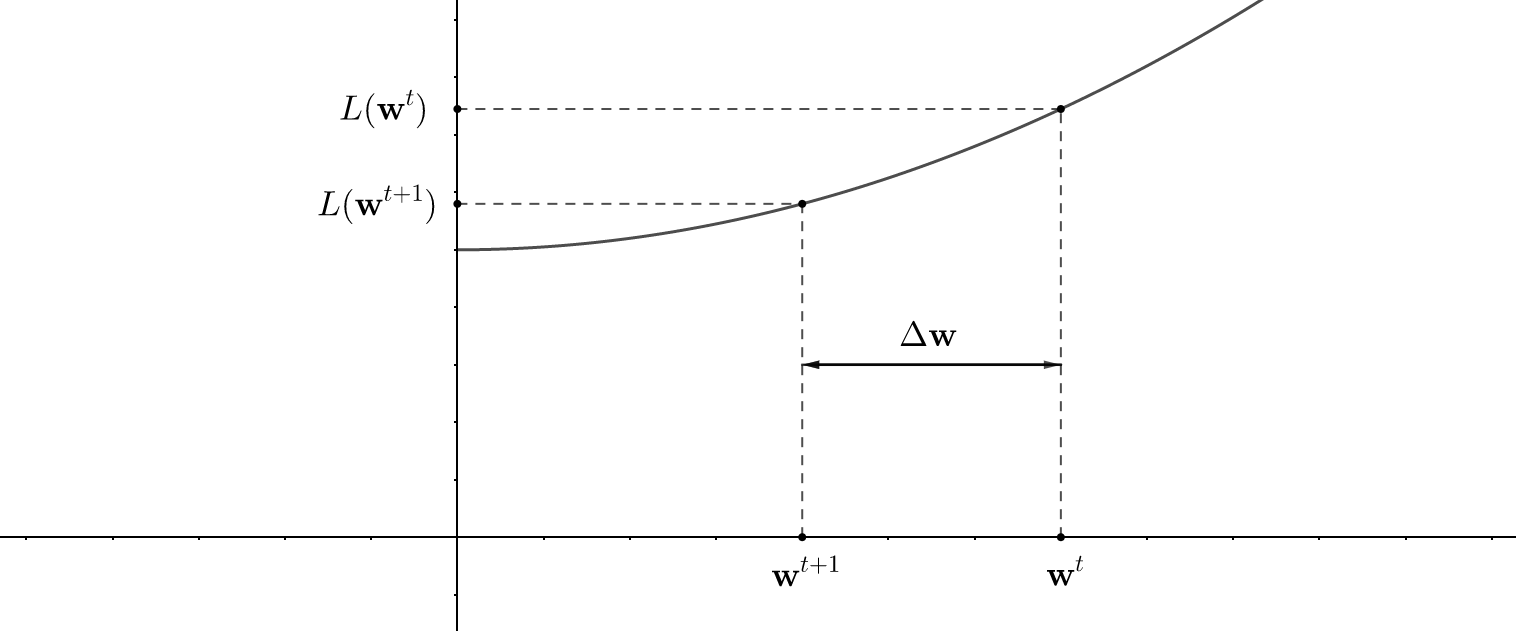
Let's say that the neural network was initialized with weights \(\textbf{w}_{0}\). Thus, to find \(L\)'s minimum, we need to move along \(\Delta \textbf{w}\) in such a way, that the next value \(L(\textbf{w}_{0} + \Delta \textbf{w})\) will be lower than the previous one: \(L(\textbf{w}_{0})\), i.e., \(L(\textbf{w}_{0}) > L(\textbf{w}_{0}+ \Delta \textbf{w})\).

For brevity, it is convenient to denote \(L(\textbf{w}_{0})\) and \(L(\textbf{w}_{0}+\Delta \textbf{w})\) as \(L(\textbf{w}^{t})\) and \(L(\textbf{w}^{t+1})\) respectively. In other words, these two values represent the loss function computed "at the current moment" (\(t\)-th iteration) and "at the next moment" (\(t+1\)-th iteration):

Since in practice \(L\) depends on millions of different arguments, it is difficult and expensive to compute its second derivatives (although some algorithms do that for more precise convergence), so we can omit them in \((1)\). Thus, using aforementioned notation we can simplify \(L\) to the following expression: \[ L(\textbf{w}^{t+1}) \approx L(\textbf{w}^{t}) + \nabla L(\textbf{w}^{t})^{\mathsf{T}} \cdot \Delta \textbf{w}^{t}; \quad \Delta \textbf{w}^{t} = \textbf{w}^{t+1} - \textbf{w}^{t} \] Then, the above condition \(L(\textbf{w}_{0}) > L(\textbf{w}_{0}+ \Delta \textbf{w}) \Leftrightarrow L(\textbf{w}^{t}) > L(\textbf{w}^{t+1})\) can be expressed as follows: \[ \Delta L = L(\textbf{w}^{t}) - L(\textbf{w}^{t+1}) = - \nabla L(\textbf{w}^{t})^{\mathsf{T}} \cdot \Delta \textbf{w}^{t} > 0 \] How to make something to be always positive? Correct! This something should be equal to something else squared! Therefore, if we assume that \(\Delta \textbf{w} = - \eta \nabla L(\textbf{w}^{t}) \) with some \( \eta \in (0, +\infty) \), then the previous expression becomes: \[ \Delta L = - \nabla L(\textbf{w}^{t})^{\mathsf{T}} \cdot (- \eta \nabla L(\textbf{w}^{t})) = \eta \cdot ||\nabla L(\textbf{w}^{t})||_{2}^{2} > 0 \quad \blacksquare \] So it is exactly what we want! Combining everything together, we have:

\[ \begin{equation} \Delta \textbf{w}^{t} = - \eta \nabla L(\textbf{w}^{t}) \Rightarrow \textbf{w}^{t+1} = \textbf{w}^{t} - \eta \nabla L(\textbf{w}^{t}) \end{equation} \]

This expression stands for the so-called gradient descent iterative optimization algorithm. The hyperparameter \( \eta \) is called the learning rate, because it regulates the speed how fast we move towards the minimum.

This method is simple in that it only suggests moving in the opposite direction of the gradient without requiring any additional computations. However, in extreme cases, the algorithm does not behave appropriately: namely, it gets stuck in local minima and slowly converges on the “flat” sections of the loss function. To help gradient descent avoid these problematic situations, the so-called momentum \( \alpha \in [0, 1) \) is introduced. This approach adds into \((2)\) an additional term that takes into account the previous weights decrement \(\Delta \textbf{w}^{t-1}\): \[ \begin{equation} \Delta \textbf{w}^{t} \equiv \textbf{w}^{t+1} - \textbf{w}^{t} = - \eta \nabla L(\textbf{w}^{t}) + \alpha \Delta \textbf{w}^{t-1} \end{equation} \] Thus, for example, when the loss function is flat over some region, we may assume that \(\Delta \textbf{w}^{t} \approx \Delta \textbf{w}^{t-1}\), so: \[ \Delta \textbf{w}^{t}(1-\alpha) \approx - \eta \nabla L(\textbf{w}^{t}) \Rightarrow \eta_{\text{effective}} \approx \dfrac{\eta}{1-\alpha} \gg \eta \quad \forall \alpha \in [0, 1) \] So the effective learning rate is accelerated by the momentum, in this case, helping the algorithm to descend faster:

Stochastic Gradient Descent

Obviously, having a large amount of training data, gradient descent will work too slowly, because every single iteration requires the loss function in \((2)\) to be computed against all training examples. Therefore, in practice, the network's weights are often updated after processing each training example one by one, so the gradient value is approximated by a gradient of the loss function calculated on only one training example. This approach is called stochastic gradient descent. The theory of stochastic approximations proves that, by observing certain requirements, the aforementioned approach converges and can be used in practice.

As a kind of compromise between the speed of convergence and the algorithm performance, the so-called mini-batch approach is often used in the industry. In this case the gradient value is computed over a small set of randomly selected training examples called batch or simply \(\pi\), so the data set is divided into batches \(\mathcal{D} = \lbrace \pi_{1}, \ldots, \pi_{t}, \ldots \rbrace\). With that said, the gradient averaged for a batch is used to update the weights. Further, this process should be repeated for a new batch of examples: \[ \Delta \textbf{w}^{t} = -\eta \nabla L(\textbf{w}^{t}); \quad \nabla L(\textbf{w}^{t}) = \dfrac{1}{|\pi_{t}|} \sum_{i\in \pi_{t}} \nabla L_{i}(\textbf{w}^{t}) \] , where \(|\pi_{t}|\) is \({\pi}_{t}\)-th batch size and \(\nabla L_{i}\) is the gradient computed for \(i\)-th training example from this batch.

Gradients Calculation

Now that we know everything that is needed regarding the theoretical part, nothing prevents us from putting this knowledge into practice and delineate the sketch of the neural network weights update algorithm. As we discussed in the section above, we first need to compute the respective gradients. All calculations below are based on processing only one input example.

Output Layer

Let's start with the output layer, which is made of \(n\) neurons. For simplicity, let's consider some \(m\)-th neuron with an activation function \(\varphi_{l}\)² located in between of the layer. In the previous post, we decided to denote the output signal of this neuron \(y_{l}^{m}\) as follows: \[ y_{l}^{m} = \varphi_{l} (z_{l}^{m}) = \varphi_{l} \left (\sum_{j=1}^{n} w_{l}^{m,j} \cdot y_{l-1}^{j} + b_{l}^{m} \right ) \] According to the same notation, this neuron's \(i\)-th weight is denoted as \(w_{l}^{m,i}\):

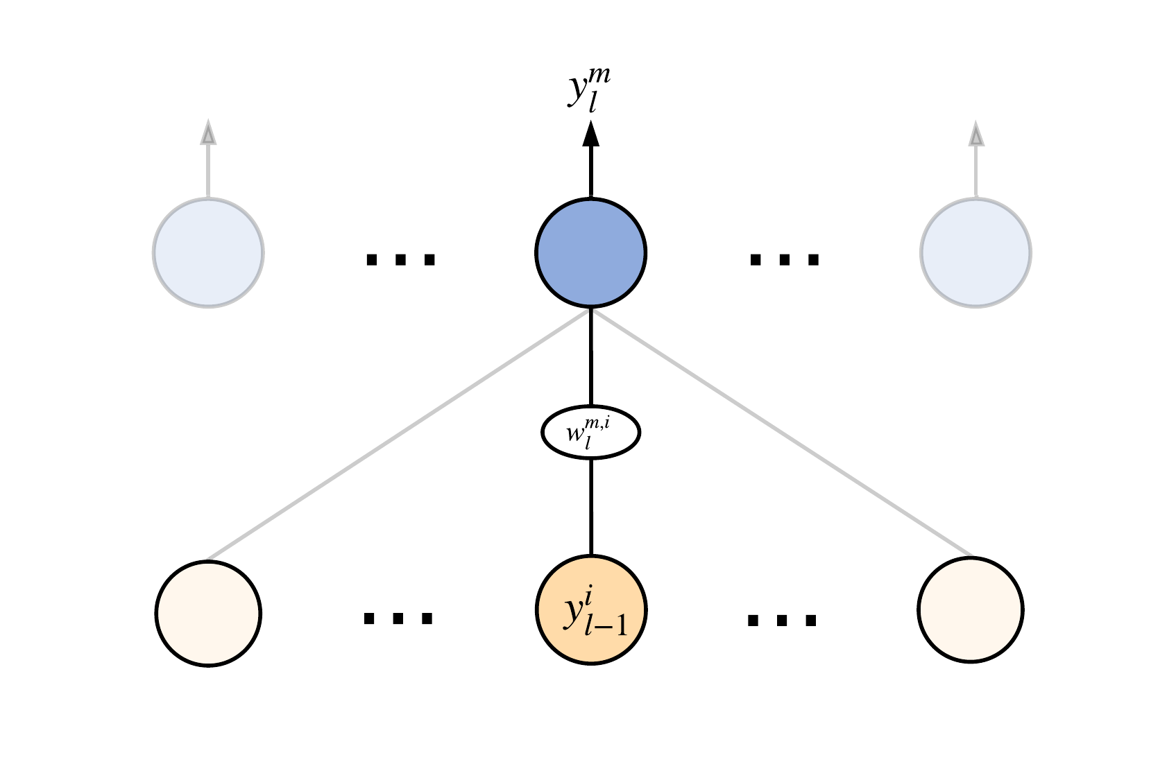
Based on expression \((2)\), we have to compute the gradient with respect to the corresponding weight. Let's denote the \(w\)-component of the loss function's gradient as \(\nabla w\). Utilizing the chain rule and the neuron's activation formula above, we have: \[ \nabla w_{l}^{m,i} = \dfrac{\partial L}{\partial w_{l}^{m,i}} = \underbrace{\left. \dfrac{\partial L}{\partial y} \right |_{y=y_{l}^{m}}}_{L'} \cdot \underbrace{\left. \dfrac{\partial y_{l}^{m}}{\partial z} \right |_{z=z_{l}^{m}}}_{\varphi'} \cdot \left. \dfrac{\partial z_{l}^{m}}{\partial w} \right |_{w=w_{l}^{m,i}} \] Since \(z_{l}^{m}\) is a linear function, it is not hard to compute the last term: \[ \left. \dfrac{\partial z_{l}^{m}}{\partial w} \right |_{w=w_{l}^{m,i}} = y_{l-1}^{i} \] After combining everything together we finally have: \[ \begin{equation} \nabla w_{l}^{m,i} = L' \cdot \varphi' \cdot y_{l-1}^{i}; \, \nabla b_{l}^{m,i} = L' \cdot \varphi' \end{equation} \] Thus, the gradient \(\nabla w_{l}^{m,i}\) is proportional to the underlying neuron's output signal \(y_{l-1}^{i}\). This is why to calculate gradients for all weights of the output layer, we have first to calculate the output signals of all neurons of the network. For example, in the case of a quadratic loss function and the sigmoid activation function we'll get (omitting the layer index \(l\)): \[ \begin{equation} L^{m} = \dfrac{1}{2}||y^{m}-t^{m}||_{2}^{2}; \, \varphi(x) = \sigma (x) \Rightarrow \nabla w^{m,i} = (y^{m}-t^{m}) (1-y^{m}) y^{m} y_{l-1}^{i} \end{equation} \] If the last layer is a softmax layer and the categorical cross-entropy is used, we can show that using the equality \(\sum_{i}t^{i} = 1\), the gradient can be computed as: \[ L = - \vec{t} \log{\vec{y}}; \, \varphi(x) = \text{softmax} (x) \Rightarrow L = -\sum_{i=1}^{n} t^{i} \log{y^{i}}; \, y^{i} = \dfrac{e^{z^{i}}}{e^{z^{m}}+\rho}; \, \rho = \sum_{i \ne m}^{n} e^{z^{i}} \Rightarrow \] \[ \dfrac{\partial L}{\partial z^{m}} = -1 \cdot \left [ t^{m} \dfrac{\partial}{\partial z^{m}} \left ( \dfrac{e^{z^{m}}}{e^{z^{m}}+\rho}\right) + \sum_{k \ne m}^{n} t^{k} \dfrac{\partial}{\partial z^{m}} \left ( \dfrac{e^{z^{k}}}{e^{z^{m}}+\rho}\right) \right ] = \] \[ = - t^{m} \dfrac{\rho}{\rho + e^{z^{m}}} + \sum_{k \ne m}^{n} t^{k} \dfrac{e^{z^{m}}}{\rho + e^{z^{m}}} = - t^{m} \dfrac{\rho}{\rho + e^{z^{m}}} + e^{z^{m}} \dfrac{1 - t^{m}}{\rho + e^{z^{m}}} = y^{m} - t^{m} \Rightarrow \] \[ \begin{equation} \nabla w_{l}^{m,i} = (y^{m}-t^{m}) y_{l-1}^{i} \end{equation} \] Here is the answer to the question why softmax and cross-entropy works better for classification rather than sigmoid and quadratic loss function. Comparing \((5)\) and \((6)\), it is easy to see, that for \(y^{m} \approx 0\) or for \(y^{m} \approx 1\) \(\rightarrow \nabla w_{l}^{m,i} \approx 0\). This is one of the manifestations of the so-called vanishing gradient problem. In the case of the softmax activation, regardless of \(y^{m}\) value, gradient value \(\nabla w_{l}^{m,i}\) depends only on the absolute difference between the expected and the produced signals. This property of the softmax, of course, helps the training to be more efficient in terms of convergence speed.

Hidden Layers

What about the underlying hidden layers' neurons? Actually - nothing changes. We need to compute their gradients absolutely similarly to the calculations we've just done above. For brevity, in \((4)\), let's denote neuron-specific term \(L' \varphi'\) as \(\delta^{m}_{l}\): \((4) \Leftrightarrow \nabla w^{m,i}_{l} = \delta^{m}_{l} y^{i}_{l-1}\). Now, let's take a look at the \(i\)-th neuron from the penultimate \(l-1\)-th layer:

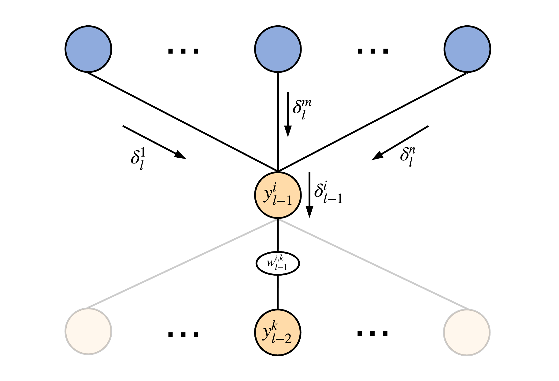
From the point of view of its operation, this neuron is no different from its neighbors above, therefore the expression for its activation function is equal to: \[ y^{i}_{l-1} = \varphi_{l-1} \left (\sum_{k=1}^{n} w_{l-1}^{i,k} \cdot y_{l-2}^{k} + b^{i}_{l-1} \right ) \] Thus, the gradient for this neuron's \(k\)-th weight \(w_{l-1}^{i,k}\) is given as follows: \[ \nabla w_{l-1}^{i,k} = \dfrac{\partial L}{\partial w_{l-1}^{i,k}} = \sum_{j}^{n} \left ( \left. \dfrac{\partial L}{\partial y } \right |_{y=y_{l}^{j}} \cdot \left. \dfrac{\partial y_{l}^{j}}{\partial z} \right |_{z=z_{l}^{j}} \cdot \left. \dfrac{\partial z_{l}^{j}}{\partial w} \right |_{w=w_{l-1}^{i,k}} \right ) \] The first two elements of the product inside the parentheses are just introduced term \(\delta^{m}_{l}\), so: \[ \nabla w_{l-1}^{i,k} = \sum_{j}^{n} \left ( \delta_{l}^{j} \cdot \left. \dfrac{\partial z_{l}^{j}}{\partial w} \right |_{w=w_{l-1}^{i,k}} \right ) \] Writing down the expression for \(z_{l}^{j}\), we immediately get: \[ z_{l}^{j} = \sum_{s=1}^{n_{l-1}} w_{l}^{j,s} \cdot y_{l-1}^{s} + b^{j}_{l} \Rightarrow \nabla w_{l-1}^{i,k} = \sum_{j}^{n} \left ( \delta_{l}^{j} \cdot w_{l}^{j,i} \cdot \left. \dfrac{\partial y_{l-1}^{i}}{\partial w} \right |_{w=w_{l-1}^{i,k}} \right ) \] Now, since \(w_{l-1}^{i,k}\) belongs only to neuron \(y_{l-1}^{i}\), the last element of the product also depends only on this neuron. Therefore, we can factor it out giving: \[ \nabla w_{l-1}^{i,k} = \left ( \sum_{j}^{n} \delta_{l}^{j} \cdot w_{l}^{j,i} \right ) \cdot \left. \dfrac{\partial y_{l-1}^{i}}{\partial w} \right |_{w=w_{l-1}^{i,k}} \] , where the last derivative can be computed similarly to the case of the output neurons explained above, so there is nothing new: \[ \begin{equation} \left. \dfrac{\partial y_{l-1}^{i}}{\partial w} \right |_{w=w_{l-1}^{i,k}} = \varphi_{l-1}' \cdot y_{l-2}^{k} \Rightarrow \nabla w_{l-1}^{i,k} = \left ( \sum_{j}^{n} \delta_{l}^{j} \cdot w_{l}^{j,i} \right ) \cdot \varphi_{l-1}' \cdot y_{l-2}^{k} \end{equation} \] Similarly we can compute the update for the bias \(b_{l-1}^{i}\): \[ \nabla b_{l-1}^{i} = \left ( \sum_{j}^{n} \delta_{l}^{j} \cdot w_{l}^{j,i} \right ) \cdot \varphi_{l-1}' \] Here comes the pattern...

Backpropagation

If you look closely at \((4)\) and \((7)\), you'll notice that they're similar enough. They both are made of the following three terms: \[ \begin{equation} \nabla w_{l}^{m,i} = \Delta_{l}^{m} \cdot \varphi_{l}' \cdot y_{l-1}^{i} \end{equation} \] They both are proportional to the following two terms:

\(\Delta_{l}^{m}\) - aggregated error. This error doesn't depend on the weight, which is being considered. As we just found out, in the case of the output layer neurons, \(\Delta_{l}^{m}\) equals to \(L'\equiv \partial L / \partial y_{l}^{m} \). For the hidden neurons, this term equals to the sum of errors from the overlying neurons, multiplied by the weights of their connections with the considered neuron: \(\Delta_{l}^{m} = \sum_{j}^{n} \delta_{l}^{j} \cdot w_{l}^{j,m}\).

\(\varphi_{l}'\) - neuron-specific error. Depends only on the neuron's activation function value.

\(y_{l-1}^{i}\) - connection-specific error. The term that corresponds to the input signals, which are passed through the respective connection. For the input layer this term is equal to the respective input signal: \(y_{0}^{i} \equiv x^{i}\).

So, we've just connected everything that happens during the calculation of the gradient: from the moment of receiving the input signal and computing the loss function value for in this example, to the moment when this error, starting from the output layer, is propagated back down the network transforming from layer to layer. Hence the name - backpropagation algorithm. The history of this algorithm was described in this post.

This series of posts, describing the theoretical foundations of neural networks, as I said earlier, won't deal with purely practical questions, such as the implementation of the training algorithm. Because, first of all, it is already beautifully described in many other sources. Thus is a matter of taste. And secondly, it does not change the basic essence of how neural networks are trained. That is why, as an intermediate result of our conversation today, I would like to present the general scheme of training using the backpropagation algorithm in tandem with SGD. This algorithm is a summary of all calculations, which were given above:

Almost all feedforward neural networks are trained this way. Algorithms differ in implementation and in multiple optimizations, which are needed to speed up computations and save the resources.

...

This is all I wanted to highlight in this post. Thank you! See you next time, when we'll be talking about another important aspect of the neural networks training - regularization.

Notes

---

1. Another way to denote \(p_{\textbf{w}}(\mathcal{D})\) is \(p(\mathcal{D}|\textbf{w})\), but we will use the first option in this post for consistency.↩
2. We assume, that every \(l\)-th layer has \(n_{l}\) neurons with the same activation function \(\varphi_{l}\).↩

---