Applied Math.
Part II: Derivative.
Foreword
In the previous post we started talking about applied mathematics, and touched upon some basic concepts, and today our topic is derivatives.
By the end of XVII century, Isaac Newton discovered laws of mechanics, found the law of universal gravitation and built the mathematical theory, helping reduce "uneven to uniform" and "heterogeneous to homogeneous". Simultaneously with Newton, the German mathematician Gottfried Wilhelm Leibniz was studying how to draw tangents to curves. Independently of each other, almost at the same time, Leibniz and Newton discovered calculus. Leibniz used the notation that turned out to be so convenient, that it is still used to this day.
The new math created by Newton and Leibniz consisted of two major parts: differential and integral calculus. The first part in its basis has a straightforward idea: any small changes in continuous functions can be approximated as linear. The idea of integral calculus is based on the approach of using these small linear approximations to work with some complex, irregularly varying functions.
In this post, I would like to talk only about the two most essential parts of the differential calculus: derivative and differential. To be more precise, we will define the derivative and explain its geometric meaning, find out what the differential is and how it differs from the derivative. We also will be talking about how derivatives work for functions of several variables and will thoroughly consider how all this can be used for real-life applications.
The material will become more difficult from section to section, therefore feel free to skip what you think is unnecessary or too complicated. Further, all the same principles will be used for the notation which were described in the first part of this series of posts. So, let's get started!
The Idea and Definition
Nikolai Lobachevsky said: "There is no branch of mathematics, however abstract, which may not some day be applied to phenomena of the real world". So does derivative. The concept of the derivative pervades all modern science, including physics, chemistry, economics and whatever you can imagine, so let's consider the following example. A car moving on a straight road from point \(A\) to point \(B\) with a distance of 100 kilometers between them. The question: "What was the average car speed if it finished the trip within 2 hours?" Of course, you have already answered the question: \(\overline{v} = \dfrac{S}{t} = \dfrac{100}{2} = 50\) km/h. But what if we would like to study the average speed of the car at each point of its path? Well, as you might have guessed, we need to know the car coordinate function \(s(t)\): the dependency of the coordinate \(s\) on time \(t\). Thus, more formally, between any two points \(s_{1},s_{2}\), where the car was at the moment of time \(t_{1}\) and \(t_{2}\) respectively, the average speed can be estimated using the next approximation: \[\overline{v} = \dfrac{s_{2} - s_{1}}{t_{2} - t_{1}}\]
The smaller the difference between these two time points - the better the above approximation is. So, finally, the instant car speed is becoming equal to the limit: \[v(t) = \lim_{\Delta t \rightarrow 0} \dfrac{\Delta s}{\Delta t}\]
That was an illustration of how an idea of the derivative had apparently appeared in Newton's mind, when he was studying the laws of kinematics. Therefore, the derivative is just a name for the following limit:
Consider a function \(f \, : \, [a, \, b] \rightarrow \mathbb{R}\) and a point \(x_{0} \in [a, \, b]\). If the following finite limit exists: \[\lim_{x\rightarrow x_{0}} \dfrac{f(x)-f(x_{0})}{x-x_{0}}\] , then this limit is called the derivative of the function \(f(x)\) at \(x_{0}\) and denoted by the prime symbol \(f'(x_{0})\).
If the above limit exists at each point of the interval \([a, \, b]\), then the mapping \(x\mapsto f'(x)\) appears. This new function is also called the derivative and denoted similarly: \(f'(x)\).
As you've just noticed, the denominator of the above expression, the argument increment \(\Delta x\) tends to zero, therefore, for the limit to exist, its numerator must tend to zero as well. It means that \(f(x_{0}) = \lim_{x \to x_{0}} f(x)\) and this, in turn, guarantees, that the function is continuous at \(x_{0}\). However, the converse of this fact is false, it just does not work backwards: the fact that the function is continuous does not necessarily lead to the derivative existence. Here is an example: the absolute value function \(|x|\) at \(0\).
Using this definition, formulas for all basic function derivatives can be obtained.
Geometrical Meaning
Another way to understand what the derivative is and how it works is to consider a geometric example of tangent of curves1.
The figure above depicts the so-called tangent \(\tau\) and secant \(s\) lines for some function \(f\) at some point \(x_{0}\). There are also shown the increments of the function and argument: \(\Delta f\) and \(\Delta x\) respectively.
In the general two-dimensional case, the tangent line equation is represented as follows: \[\tau(x)=A(x-x_{0})+B\]
Since by the definition of the tangent line \(\tau(x_{0}) = f(x_{0})\), then, plugging it into the expression above, we get: \(B = f(x_{0})\). Moreover, using purely geometric considerations, we can calculate the slope coefficient \(A\) of the secant line: \(A = \tan(\alpha) = (f(x)-f(x_{0}))/(x-x_{0}) = \Delta f / \Delta x\); this slope is equivalent to the angle \(\alpha\) that is shown in grey in the figure. The same figure also shows, that in the extreme case, when \(\Delta x \to 0\), the function increment also tends to zero \(\Delta f \to 0\). Thus, the ratio between function and argument increments, following the definition, approaches the value of the derivative at \(x_{0}\): \[A \xrightarrow[]{} \lim_{\Delta x\rightarrow 0} \dfrac{\Delta f}{\Delta x} = f'(x_{0})\]
Voila! On the two-dimensional plane, the derivative of a function of one variable2 at a point equals to the angle of inclination of the tangent line to this function at that point.
Thus, in the case with the car from the example above, where speed is the derivative of the coordinate function, we have that the instant speed \(v(t)\) is equal to the slope of the coordinate function \(s(t)\) at the same moment of time. Consequently, the steeper the slope, the greater the speed.
Differential
The concept of the derivative is closely intertwined with the concept of the differential of a function. To understand what the differential is, firstly, it is better to recall what linear mappings are, and, secondly, what a little-o function is.
Let's start from linear mappings. In simple words, it is a generalization of linear function to extend its properties on more domains and objects such a function may operate on. In terms of geometry, linear mappings are those mappings, which stretch and/or rotate vectors, preserving the dot product. Linear mappings are usually denoted as \(L\). In one-dimensional case, \(L\) is a linear continuous function \(x \mapsto \alpha \cdot x\), where \(\alpha \in \mathbb{R}\) is a number.
What does little-o notation mean? If we have two functions \(f\) and \(g\), then \(f\) is little-o of \(g\) for \(x \rightarrow x_{0}\), if \(g\) decreases much slower then \(f\), while approaching \(x_{0}\). This is usually denoted as follows: \(f(x) = o(g(x))\). Often, mathematicians read it as "\(f\) is infinitesimal with respect to \(g\)". More formally, the definition is always considered at some point \(x_{0}\), which belongs to both functions' domains, so the expression \(f(x) = o(g(x))\) can be easily substituted by the following limit:
\[\lim_{x \rightarrow x_{0}} \dfrac{f(x)}{g(x)} = 0 \Leftrightarrow f(x) = o(g(x)),\, x \rightarrow 0\]For instance, \(x^3 = o(x)\) when \(x \to 0\). Usually, this notation is used, when functions are being approximated. For example, near zero, sine behaves like a linear function, and this fact might be written like this: \(\sin(x) = x + o(x), \,\, x \rightarrow 0\). This is it! Now we can move forward to the differential.
The concept of the differential of a function appeared, when mathematicians were trying to strictly define the idea of function differentiability. Under what conditions can we be sure, that some function has the derivative at some point? In fact, after a lot of research, it was shown that in order for a function to have a derivative, it suffices, that it can be linearly approximated at this point. It means that the function should have a tangent at that point. Thus, more formally:
A function \(f \, : \, U(x_{0}) \rightarrow \mathbb{R}\), defined on some neighborhood of a point \(x_{0} \in \mathbb{R}\), is called differentiable at this point, if there exists a linear mapping \(L \, : \, \mathbb{R} \rightarrow \mathbb{R}\), that for the neighborhood \(U(x_{0})\), the following is correct: \[f(x_{0}+h) = f(x_{0}) + L(h) + o(h), \qquad h \rightarrow 0 \] , where \(h \in \mathbb{R}\) is a small argument increment. If such a mapping exists, it is called the differential of the function \(f\) at the point \(x_{0}\).
The differential is a function, or more precisely - a linear mapping - and this is extremely important. There are many ways to denote the differential, but I prefer the following one: \(df(x_{0},h)\). Why? First of all, because it highlights that the differential is a function, and secondly that this function depends on both point and argument increment value. But for brevity, we will use just \(df\): the shortest and probably the most popular way of doing this.
How is this related to the derivative? There is a theorem, connecting all these three definitions: differential, derivative, and differentiability:
Assume \(f \, : \, [a, \, b] \rightarrow \mathbb{R}\) and a point \(x_{0} \in [a, \, b]\). Function \(f(x)\) has a derivative \(f'(x_{0})\) at \(x_{0}\) if and only if there exists the differential \(df\) (i.e., \(f\) is differentiable), in so doing, \(df(x_{0},h) \equiv df = f'(x_{0})h\).
The argument increment \(h\) is usually considered arbitrary. The differential, being a linear mapping, changes these increments as follows: it stretches them in proportion to the value of the derivative at a given point.
If \(h\) is small enough and we can neglect the error \(o(h)\), then the differential of a linear function \(y=x\) is given by: \(dx \equiv d(y) = d(x) = (x)'h = 1\cdot h\). Thus, this differential is equal to its argument increment \(h\). Therefore, the above expression for the differential of an arbitrary function \(f\) can be easily rewritten: \(df = f'(x)h \Leftrightarrow df = f'(x)dx\), which is why, sometimes the derivative is denoted by: \[f'(x) = \dfrac{df}{dx}\]
Although it is not a strict definition and it can lead to the erroneous conclusions, so I do advise you to use this only as a notation and not as a formula. This is how more than 300 hundred years ago the Leibniz's notation appeared.
To summarize, the differential is a linear part of the function increment, connecting it with the argument increment through the derivative of this function: \(df = f'(x)dx\).
Higher-order Derivatives
Of course, it is absolutely fine, being functions, for some derivatives to have their own derivatives as well. The definition of the derivative of an arbitrary order is defined recurrently:
\(n\)-th-order derivative is defined through the \(n-1\)-th derivative, i.e., \(f^{(n)}(x) = (f^{(n-1)})'(x)\).
For example, for a cubic function \(y = x^{3}\), its third-order derivative is given by:\(y''' = (x^{3})'''=(3x^{2})''=(6x)'=6\). In Leibniz's notation \(n\)-th-order derivative symbol is written as follows: \(\dfrac{d^{n}f}{dx^{n}}\).
Bearing in mind the same logic, one can introduce the concept of the higher-order differential. For example, the second-order differential is defined by the following expression: \[d^{2}f(x_{0}) = f''(x_{0})(dx)^{2} = f''(x_{0})dx^{2}, \quad dx^2 \equiv (dx)^2 \] Thus, for example, for a linear function \(y = x\), its second differential equals zero: \(d^{2}y = d^{2}x = 0 \cdot (dx)^{2} = 0\).
Just like most things in math, higher-order derivatives also carry the physical meaning. For example, in the case of a car, its speed is the derivative of the car's distance function. So, the car's acceleration is the derivative of the speed, that is, the second-order derivative of the distance function. We will discuss that later in this post. Such connections between different concepts are incredibly important for physics. It is also impossible to overemphasize the importance of the second-order derivatives for the convex analysis, where the derivatives can be used, for instance, to determine whether a given function is convex.
Multivariable Functions and the Partial Derivatives
The world is not limited only by single-variable functions: many things may depend on many other things. For example, the indoor temperature of your house depends on the outside temperature, the materials of walls, floors, ceilings and so on. Such complex dependencies are called multivariable functions or functions of several variables.
Speaking rigorously:
Consider two Euclidean spaces \(\mathbb{R}^{n}\) and \(\mathbb{R}^{m}\). If there exists an open connected set (usually called a region) \(\mathcal{D} \subset \mathbb{R}^{n}\), then a mapping \(f \, : \, \mathcal{D} \rightarrow \mathbb{R}^{m}\) is called a multivariable function, that maps each point \(\mathbf{x} \in \mathcal{D}\) to its \(m\)-dimensional image.
That is, such a function transfers points from the \(n\)-dimensional space to the \(m\)-dimensional one. No more, no less.
Almost all the definitions/ideas/notations/theorems in single-variable function theory might be applied for the multivariable functions. Moreover, even notation will not change much. For example, all modulus signs \(||\) should be replaced with the respective Euclidean norm \(\lVert \cdot \rVert\).
The definition of the derivative for multivariable functions can be introduced through the definition of the partial derivative. Usually, a scalar-valued function \(f \, : \, \mathbb{R}^{n} \rightarrow \mathbb{R}\) is considered for simplicity. In this context, the word "partial" means that all function arguments are fixed at some point \(\mathbf{x}_{0} = (x_{1}, x_{2}, \dots, x_{n}) \in \mathbb{R}^{n}\) (multidimensional objects will be further highlighted in bold) except for a single argument \(x_{i}\), which is changed. Thus, similarly to the single-variable derivative definition, we have:
If the following limit exists: \[\lim_{\Delta x_{i} \rightarrow 0} \dfrac{f(x_{1}, \dots , x_{i}, \dots x_{n})-f(x_{1}, \dots,x_{i} + \Delta x_{i} , \dots, x_{n})}{\Delta x_{i}}\] , then this limit is called the derivative of the function \(f(\mathbf{x})\) at \(\mathbf{x}_{0}\) with respect to the variable \(x_{i}\) and denoted by the following symbol: \(\dfrac{\partial f}{\partial x_{i}}\).
That is, in simple words, the partial derivative is a regular derivative, but computed for the multivariable function, whose arguments are "frozen" except for a single considered variable.
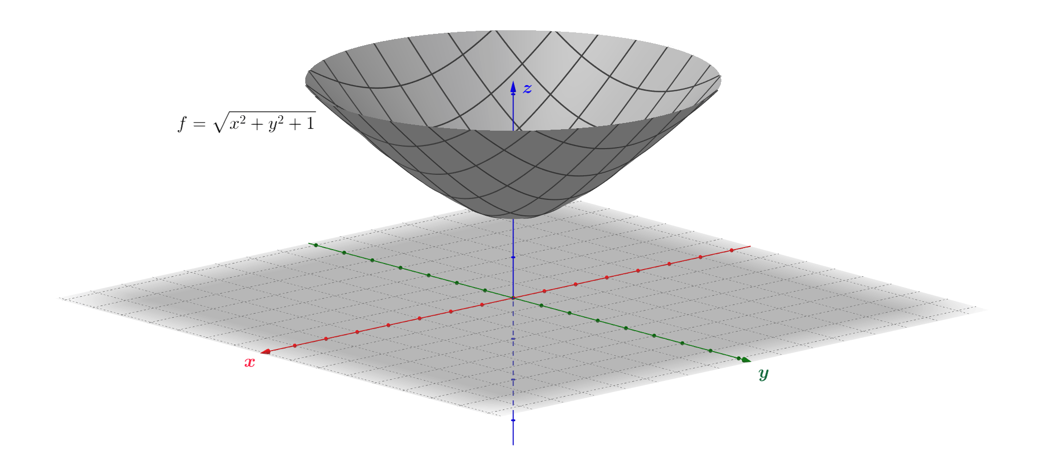
Let's consider function \(f\) from the above illustration: \[f \, : \, (x,y) \mapsto (x,y,\sqrt{x^{2}+y^{2}+1}) \]
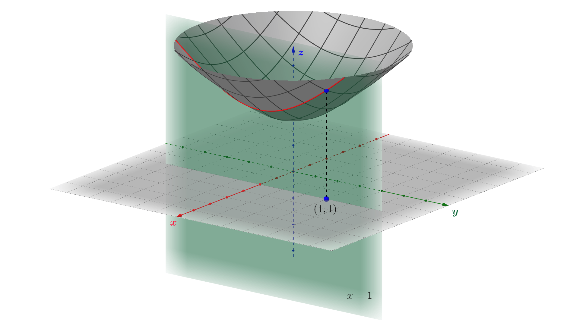
For example, let's assume \(x = 1\), i.e., "fix" variable \(x\). Geometrically it means that we need to draw a plane \(x = 1\). Then, the intersection of that plane and the function surface will "cut out" a curve \(y \mapsto (1,y,\sqrt{y^{2}+2})\) (the red curve in the figure below). Thus, for the \(y\)-partial derivative of \(f\), we have to consider a function \(\sqrt{y^{2}+2}\). For example, at point \((1,1)\), this partial derivative is given by: \[ \dfrac{\partial f}{\partial y} = \left.\dfrac{d(\sqrt{y^{2}+2})}{dy}\right|_{y=1} = \left.\dfrac{y}{\sqrt{y^{2}+2}}\right|_{y=1}=\dfrac{\sqrt{3}}{3} \]
Also, partial derivatives can be applied multiple times with respect to different variables; these derivatives are called mixed partial derivatives. Here is an example. Given a scalar-valued function \(f = x^{2} / y \), the mixed partial derivative with respect to the variables \(x\) and \(y\) will be: \[ \dfrac{\partial^{2} f}{\partial x \partial y} = \dfrac{\partial}{ \partial x} \dfrac{\partial (x^2/y)}{\partial y} = \dfrac{\partial (-x^{2}/y^{2})}{ \partial x} = \dfrac{-2x}{y^{2}} \]
Differential of a Scalar Function
The question of the differentiability of functions of several variables, as in the one-dimensional case, is connected with the concept of the differential. The sufficient condition for the differentiability might be written as follows:
Assume \(\mathcal{D} \in \mathbb{R}^{n}\) is a region, where a function \(f \, : \, \mathcal{D} \rightarrow \mathbb{R}\) is defined. If all first-order partial derivatives exist and they are continuous at \(\mathbf{x}_{0}\), then this function is differentiable at this point.
However, the necessary condition is the following:
If \(f\) is differentiable at \(\mathbf{x}_{0}\), then all partial derivatives of \(f\) exist, and the function increment can be expressed in the form: \[ f(\mathbf{x}_{0}+\Delta\mathbf{x})-f(\mathbf{x}_{0})=\underbrace{\sum_{i=1}^{n}\dfrac{\partial f}{\partial x_{i}}(\mathbf{x}_{0}) \Delta x_{i}}_{=df(\mathbf{x}_{0}, \Delta \mathbf{x})} + o(\lVert \Delta \mathbf{x} \rVert), \qquad \Delta \mathbf{x} \rightarrow 0 \] In the case when all variables are independent and the argument increment is infinitesimal, then all \(\Delta x_{i} = dx_{i}\).
By the way, if all partial derivatives of \(f(\mathbf{x})\) exist at some point \(\mathbf{x}_{0}\), then this function is called smooth.
In the more general case, when \(\mathbb{R}^{n} \rightarrow \mathbb{R}^{m}\) functions are considered, the differential, being a linear mapping, becomes a matrix operator, represented through the Jacobian matrix, that acts on the argument increment vector \(\Delta \mathbf{x}\). Thus, it takes \(\Delta \mathbf{x}\) as input and with some error \(o(\lVert \Delta \mathbf{x} \rVert)\) produces as output a vector of the function increment: \[df_{\mathbf{x}_{0}}: \Delta \mathbf{x} \mapsto \Delta \mathbf{f}\] The way how this transformation is performed also depends on the considered point \(\mathbf{x}_{0}\):
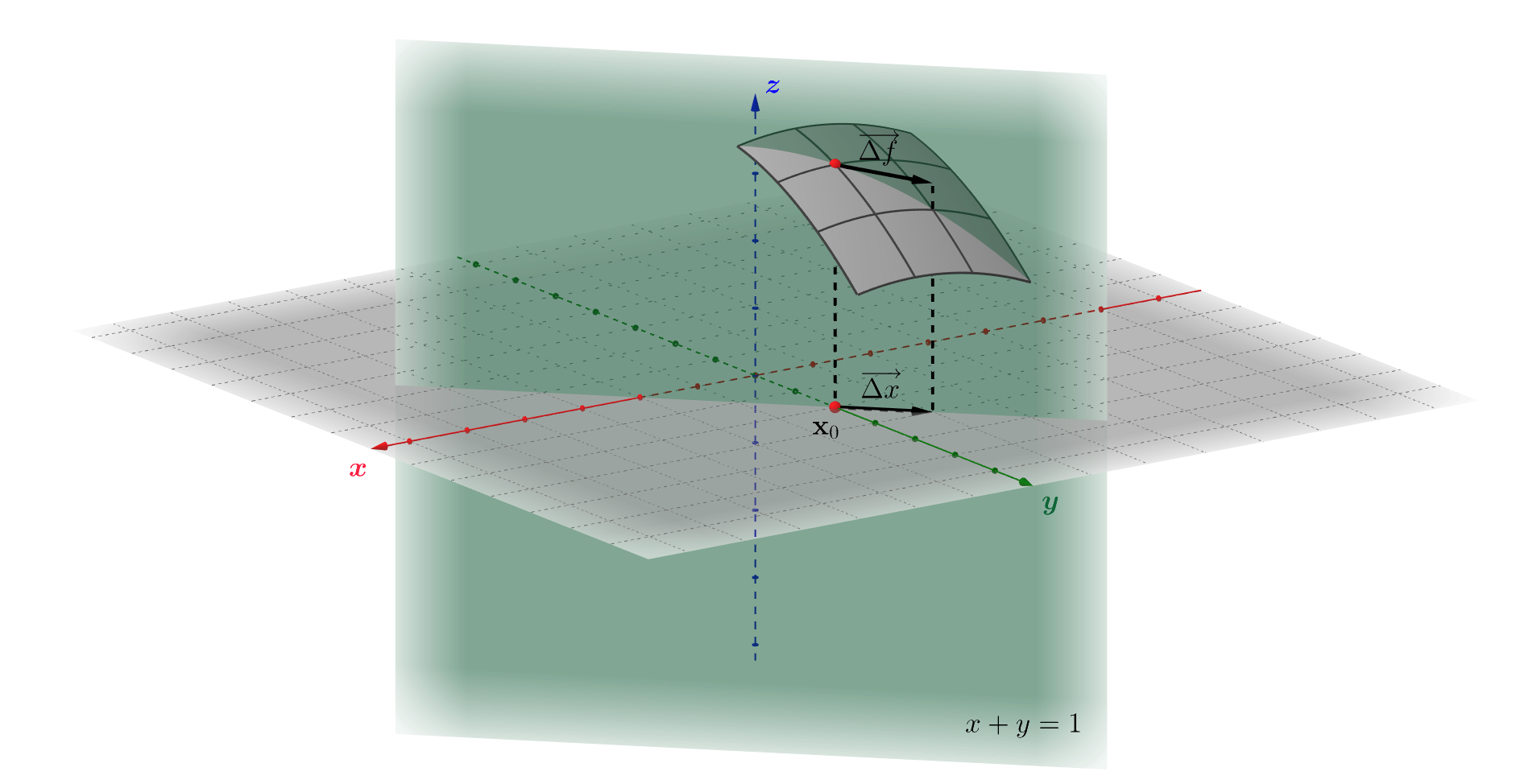
Moving too fast? Well, let's take a break and try to see how it works in practice. Let's consider as an example function \(f = 1 - 0.2\cdot(x^{2}+y^{2})\) from the figure above. Since \(f\) is a \(\mathbb{R}^{2} \rightarrow \mathbb{R}^{3}\) function, its differential \(df\) is a \(3 \times 2\) linear operator: \[ f \equiv \begin{bmatrix} f_{1} \\ f_{2} \\ f_{3} \end{bmatrix} = \begin{bmatrix} x \\ y \\ 1 - 0.2\cdot(x^{2}+y^{2}) \end{bmatrix} \Rightarrow df = \begin{pmatrix} \frac{\partial f_{1}}{\partial x} & \frac{\partial f_{1}}{\partial y} \\ \frac{\partial f_{2}}{\partial x} & \frac{\partial f_{2}}{\partial y} \\ \frac{\partial f_{3}}{\partial x} & \frac{\partial f_{3}}{\partial y} \end{pmatrix} = \begin{pmatrix} 1 & 0 \\ 0 & 1 \\ -0.4x & -0.4y \end{pmatrix} \] \[ df_{(1,1)} \cdot \Delta \mathbf{x} \equiv df_{(1,1)} \cdot \begin{bmatrix} dx \\ dy \end{bmatrix} = \begin{bmatrix} dx \\ dy \\ -0.4(xdx+ydy) \end{bmatrix} \] What's this about? How should it work? Well, everything is shown in accordance with the definition: the differential, in this particular case, is taking an arbitrary increment vector \(\Delta \mathbf{x} = (dx,dy, 0)\) from the \(XY\)-plane and maps it onto the tangent space of the surface (hatched gray parallelogram in the figure) made by function \(f\) in the \(3D\)-space.
During this "mapping", the original vector's direction and initial point are preserved. Why? Because if you take a look at the first two rows of the differential, then you'll see that it has exactly the same \(x\) and \(y\) coordinates: \(dx\) and \(dy\), whereas the argument increment's \(z\)-component has became non-zero: \(-0.4(xdx+ydy)\). Thus, for example at \(\mathbf{x}_{0} = (0,1)\), vector \((-1,1,0)\) will be moved and become equal to \((-1,1,-0.4)\), and it is the vector that represents an approximation of the function increment \(\Delta \mathbf{f}\). This is how the differentials work in the general case.
Gradient
The gradient is a widely spread term, which is used in calculus to represent a scalar-function derivative through all its partial derivatives being collected into a single vector.
Consider a scalar function \(f \, : \, \mathbb{R}^{n} \rightarrow \mathbb{R}\). If at some point \(\mathbf{x}_{0}\in\mathbb{R}^{n}\) all its partial derivatives \(\dfrac{\partial f}{\partial x_{i}}\) exist and they are continuous, then the gradient at point \(\mathbf{x}_{0}\) of the function \(f\) is called the following vector: \((\dfrac{\partial f}{\partial x_{1}}, \dots, \dfrac{\partial f}{\partial x_{n}})\). This vector is denoted by \(\mathrm{grad}f\) or \(\nabla f\).
The scalar multiplication of the function gradient and the argument increment, by definition, will give us an expression for the differential: \(df = \langle \mathrm{grad}f, \Delta \mathbf{x} \rangle\).
What is the gradient used for? This term was introduced in mathematics at the end of XIX century by the great Scottish physicist J. C. Maxwell. The gradient was used to simplify the description of the so-called scalar fields. The gradient is a handy tool, that might be used for studying different functions. For example - in order to find their extrema - because the gradient computed at each point indicates in its direction the greatest rate of increase of a function.
Let's not change our traditions and consider an example of the vector gradient field for the function \(f = \sqrt{x^{2}+y^{2}+1}\) defined on a square area \(X\times Y = [-1,1]\times[-1,1]\):
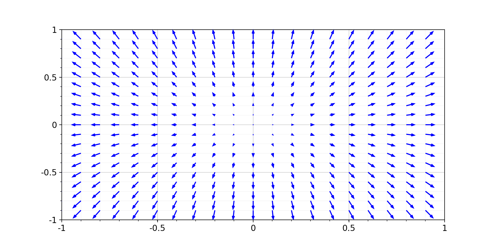
Here it is seen that starting from the origin \((0,0)\), the gradient vectors begin to grow, and they grow faster if they are farther from zero. This growth rate is shown through the norm (length) of the gradient vectors depicted.
The Hessian Matrix
There are a few more topics to be covered before proceeding to the conclusion of this post. In this section, I would like to discuss with you another important and undoubtedly convenient mathematical tool. If you need to calculate, for example, the second-order differential of some multivariable function, then it is needed to apply the differential operator to the already calculated first-order, regular differential. In the scalar-valued function case, we have to compute all possible permutations of all partial derivatives: \[ d^{2}f(\mathbf{x}_{0}) = d(df)(\mathbf{x}_{0}) = \sum_{j=1}^{n}\sum_{i=1}^{n}\dfrac{\partial^{2}f}{\partial x_{j} \partial x_{i}}(\mathbf{x}_{0})\Delta x_{j} \Delta x_{i} \] This expression can be written way simpler using the so-called Hessian matrix: \[ d^{2}f(\mathbf{x}_{0}) = \Delta \mathbf{x}^{\mathsf{T}} \cdot \mathbf{H}_{\mathbf{x}_{0}} \cdot \Delta \mathbf{x} = [\Delta x_{1}, \dots, \Delta x_{n}] \cdot \left. \begin{pmatrix}\frac{\partial^2f}{\partial x_1^{2}} & \cdots & \frac{\partial^2f}{\partial x_1 \partial x_n} \\ \vdots & \ddots & \vdots \\ \frac{\partial^2f}{\partial x_n \partial x_1} & \cdots & \frac{\partial^2f}{\partial x_n^{2}}\end{pmatrix} \right |_{\mathbf{x}_{0}} \cdot \begin{bmatrix} \Delta x_{1}\\ \vdots\\ \Delta x_{n} \end{bmatrix} \] This is a square-symmetric matrix with the size \(n\) equal to the number of function's arguments: \(\mathbf{H} \in M_{n}(\mathbb{R})\). Do not be afraid of all these intricate and intimidating matrix-vector products: it is made just for convenience and brevity. At least, because it is much easier and much more efficient for the computers (or more precisely, algorithms they use) to operate with sets of numbers rather than with each number separately.
Let's take a look at our beloved scalar function from the example 3: \(f = \sqrt{x^{2}+y^{2}+1}\). Consider this function at the point \(\mathbf{x}_{0}=(1,1)\). Because \(f\) uses two arguments, we get \(2 \times 2 \) Hessian matrix3. Usually, arguments \(x_{1}\) and \(x_{2}\) are considered as \(x\) and \(y\) variables respectively. Thus the hessian is given by: \[ \mathbf{H}_{(1,1)} = \dfrac{1}{(x^{2}+y^{2}+1)^{3/2}} \cdot \left. \begin{pmatrix}y^2+1 & -xy \\ -xy & x^2+1 \end{pmatrix} \right |_{(1,1)} = \begin{pmatrix}\dfrac{2}{\sqrt{3}} & -\dfrac{1}{\sqrt{3}} \\ -\dfrac{1}{\sqrt{3}} & \dfrac{2}{\sqrt{3}}\end{pmatrix} \] The study of the Hessian matrices at a certain point is useful to determine the extrema of multivariable functions. Let's elaborate on this.
Extremum of a Function
Despite all the beauty of the formalism of derivatives, I am deeply convinced that all this should be studied, first of all, as a tool. Furthermore, since the derivative of a function is a measure of the rate of change of this function at each point, the derivative can be used to find the special points of a function: the points at which the function takes its minimum or maximum values, or in other words, the extrema.
Firstly, it'd be useful to have a formal definition of an extremum:
Assume a function \(f \, : \, \mathcal{D} \subset \mathbb{R}^{n} \rightarrow \mathbb{R}\). Then, this function has a local minimum (or maximum) at some point \(\mathbf{x}_{0} \in \mathcal{D}\), if there exists a sphere \(S(\mathbf{x}_{0}, \delta)\) with some radius \(\delta\), that for any point inside this sphere \(\mathbf{y} \in\mathcal{D} \cap S(\mathbf{x}_{0}, \delta)\), it is correct, that \(f(\mathbf{y}) \ge f(\mathbf{x}_{0})\) (or \(f(\mathbf{y}) \le f(\mathbf{x}_{0})\)). Point \(\mathbf{x}_{0}\) that is either a maximum or minimum is called an extremum.
There exists the necessary (but not sufficient!) condition of a local extremum:
Assume a function \(f \, : \, \mathcal{D} \subset \mathbb{R}^{n} \rightarrow \mathbb{R}\), which has all its partial derivatives defined and they are continuous4. If \(f\) has a local extremum at some point \(\mathbf{x}_{0} \in \mathcal{D}\), then all the partial derivatives are equal to zero: \(\dfrac{\partial f}{\partial x_{i}} = 0 \,\, \forall i\).
For a single-variable function this statement means, that if some function \(f(x)\) has an extremum at \(x_{0}\), then \(f'(x_{0})=0\). But from the practical perspective, it is the conditions (and not consequences) under which a function may have an extremum is more useful subject to be figured out. Here comes Taylor's theorem to help us: \[ \Delta f = f(\mathbf{x}_{0} + \Delta \mathbf{x}) - f(\mathbf{x}_{0}) = \nabla f( \mathbf{x}_{0})^{\mathsf{T}} \cdot \Delta \mathbf{x} + \dfrac{1}{2!} \Delta \mathbf{x}^{\mathsf{T}} \cdot \mathbf{H}_{\mathbf{x}_{0}} \cdot \Delta \mathbf{x} + o({\lVert \Delta \mathbf{x} \rVert}^{2}) \] Therefore, near the extrema, when all partial derivatives (in accordance with the criterion above) are close to zero, we can assume that: \[ \Delta f \approx \dfrac{1}{2} \cdot d^{2}f(\mathbf{x}_{0}) = \dfrac{1}{2} \cdot \Delta \mathbf{x}^{\mathsf{T}} \mathbf{H}_{\mathbf{x}_{0}} \Delta \mathbf{x} \] , and it gives us a hint: in order to find the extrema, it is required to study the Hessian matrix behavior... Thanks to mathematicians and their research, it turned out that the hint is correct! There is the necessary and sufficient condition for an extremum:
Assume a function \(f \, : \, \mathcal{D} \subset \mathbb{R}^{n} \rightarrow \mathbb{R}\) and \(f \in C^{2}(\mathcal{D})\). Consider the Hessian matrix \(\mathbf{H}_{\mathbf{x}_{0}}\) of the function \(f\) at \(\mathbf{x}_{0}\in\mathcal{D}\): if \(\mathbf{H}_{\mathbf{x}_{0}}\) is a positive-definite (negative-definite) matrix, then \(\mathbf{x}_{0}\) is a local minimum (or a maximum). Otherwise, \(\mathbf{x}_{0}\) is not an extremum.
Sounds confusing? I'm here to help you! So first things first. The basic idea, in fact, is very logical and simple, although it is veiled by the sophisticated definition. If we consider a function near the extremum in a quadratic approximation, then this point is a local minimum if the function behaves similarly to the parabola, and a maximum, if this parabola is inverted. To better understand what is going on, let's take a look at the following example:
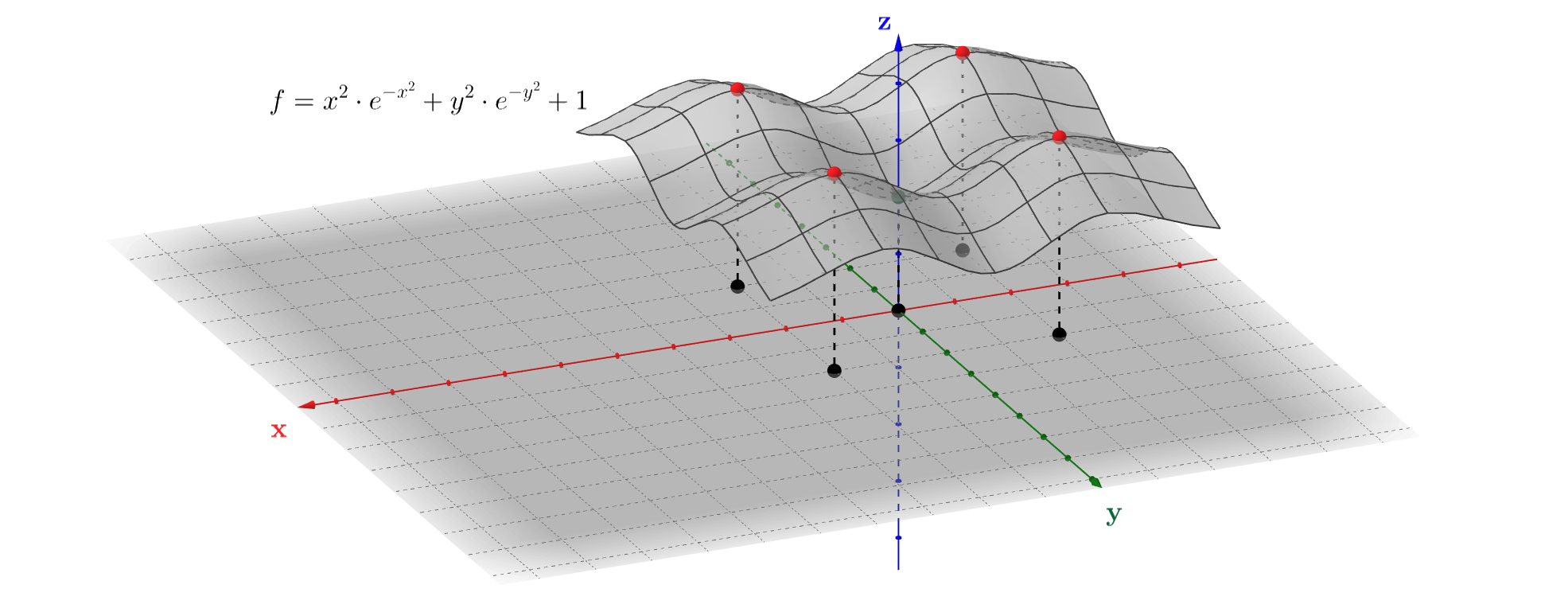
For the illustration purposes, it would be great to find all minimums and maximums of the function \(f=x^{2}e^{-x^{2}} + y^{2}e^{-y^{2}} + 1\) step by step. Firstly, we need to determine the critical points, where the partial derivatives become equal to zero: \[ \dfrac{\partial f}{\partial x} = 2x(1-x^{2})\cdot e^{-x^{2}} = 0 \Rightarrow x = {-1,0,1} \] \[ \dfrac{\partial f}{\partial y} = 2y(1-y^{2})\cdot e^{-y^{2}} = 0 \Rightarrow y = {-1,0,1} \] Thus, we have 9 potential extrema at the points where \(x\) and \(y\) coordinates can be any number from \(-1,0\) or \(1\). The next step is to investigate function behavior near the critical points. To do this, let's firstly calculate the Hessian matrix: \[ \mathbf{H} = \begin{pmatrix} 2 e^{-x^{2}} (1 - 5 x^{2} + 2 x^{4}) & 0 \\ 0 & 2 e^{-y^{2}} (1 - 5 y^{2} + 2 y^{4}) \end{pmatrix} \] To study this matrix, we can use the definition of the function increment, which we gave earlier, but with a slight reservation: at the critical points linear approximation is not enough, the second-order approximation is needed. Using the expression we've recently gotten for the second-order differential and denoting \(g(x) = 1 - 5x^{2}+2x^{4}\) for brevity, we finally have: \[ \Delta f \approx \dfrac{1}{2} \cdot [dx\,\,dy] \cdot \begin{pmatrix}2e^{-x^{2}}g(x) & 0 \\ 0 & 2e^{-y^{2}}g(y) \end{pmatrix} \cdot \begin{bmatrix} dx \\ dy \end{bmatrix} = e^{-x^{2}}g(x)(dx)^{2} + e^{-y^{2}}g(y)(dy)^{2} \] In this way, the quadratic form \(\Delta f\) is negative-definite, if both \(x=\pm 1\) and \(y=\pm 1\), because \(g(\pm 1) = -2\) and therefore \(\Delta f \approx -2e^{-1}(dx^{2}+dy^{2}) < 0\,\, \forall dx,dy \ne 0 \). Similarly, if \(x = y = 0\) \(g(0)=1\), then \(\Delta f\) is a positive-definite form, and therefore \(\Delta f > 0\,\, \forall dx,dy \ne 0 \).
In accordance with the definition, point \((0,0)\) is a local minimum, whereas four points \((1,1),\,(-1,-1),\,(-1,1),\,(1,-1)\) are local maximums respectively. At the remaining points \((0,\pm 1)\) and \((\pm 1, 0)\) we cannot definitely say that \(\Delta f\) is either positive or negative for all non-zero argument increment values. This means that these points are the so-called saddle points, that is clearly seen in the figure above. It is important to note, that instead of studying the Hessian matrix definiteness, it is possible to directly study how the function increment behaves, depending on the argument increment values. It's exactly what we've done.
All the above considerations are valid only for functions with an infinite domain. If the domain is finite, then in the case when a function has no critical points, the extrema are located at the edge points of the domain. For example, in the case of a linear function \(y=x\) defined on the positive half-plane \([0,+\infty)\), there would be a single global minimum on the left edge of the domain located at \(0\).
Summarizing the above, we can distinguish the following steps for the algorithm for finding extrema of a function:
- Calculate the partial derivatives and solve all equations \(\dfrac{\partial f}{\partial x_{i}} = 0\). If this equation system has a solution, move to the next step.
- For each critical point \(\mathbf{x}_{j}\) calculate the Hessian matrix \(\mathbf{H}_{\mathbf{x_{j}}}\).
- Having determined the matrix's definiteness using Sylvester's criterion, make a conclusion about the nature of the critical point \(\mathbf{x}_{j}\).
Applications
In general, in addition to the geometric applications, the derivative is used to solve various optimization problems: problems where, under certain conditions, it is necessary to maximize or minimize something: reduce costs, maximize profits, build the most effective rocket nozzle, train neural networks to recognize faces, and many other similar examples. In this section, I want to illustrate, that the derivative is an incredibly powerful tool. Let's start with something simple.
Example 1. Suppose we have enough building material to build a fence of length \(L\) in order to enclose a rectangular area of your country house's backyard. Of course, like anybody else, you'd like to make this area as large as possible. After all, otherwise you would not have had enough space to have a BBQ, right? So, how can we do that? Firstly, let's label both backyard's sides as \(a\) and \(b\). Since we know the expression for the perimeter \(a + b = L/2\), we have the following expression for the total square: \(S(a) = ab = a(L/2-a)\). Secondly, we need to maximize this square, using the algorithm above: \(\dfrac{d S}{d a} = 0 \Leftrightarrow L/2 - 2a = 0 \Rightarrow a_{0} = L/4\). Let's check that critical point for being a maximum: \(\dfrac{d^{2} S}{d a^{2}} = -2 < 0 \Rightarrow a_{0} \) is a global maximum, perfect! Thus, \(S_{max} = a_{0}(L/2-a_{0}) = L^{2}/16\), so, to make backyard as large as possible with the limited material for the fence - make it square-formed! Oh, had we all known that in advance...
Example 2. Imagine that a ferry runs between the mainland and the island. The ferry sails with average speed \(v\). Fuel consumption per hour can be approximated by a quadratic dependence with a fixed proportionality coefficient: \(\alpha v^{2}\). In addition, within an hour, the ferry spends another \(P\) dollars for miscellaneous expenses. We need to figure out at what speed the ferry should chose to minimize the expenses per mile. So, total expenses per hour: \(E'=P +\alpha v^{2}\), then per-mile expenses are: \(E = \dfrac{E'}{v} = \dfrac{P}{v}+\alpha v\). Let's determine the critical points: \(\dfrac{dE}{dv} = \alpha - \dfrac{P}{v^{2}} = 0 \Rightarrow v_{0} = \sqrt{\dfrac{P}{\alpha}}\). Now we have to check that it is a global minimum: \(\dfrac{d^{2}E}{dv^{2}}=\dfrac{2P}{v^{3}} > 0\). Therefore, the second derivative is always positive, at least in our circumstances. Finally, with the optimal speed \(v_{0}\) average per-hour expenses are equal to \(E'=E'(v_{0})=2P\), i.e., double miscellaneous expenses. Thus, theoretically the ferry owner has to estimate the value of \(\alpha\) to make the business more efficient.
If you want something more interesting, take a look at this post for more sophisticated example from physics, where derivatives are widely used.
...
Well, we've finally made it! Thanks for getting to the end and I hope you enjoyed it! As always, if you have any questions or comments, leave them below. In the next, third post, let's talk about integrals.
Notes
- The tangent line is a line that passes through a point of the curve and coincides with it at this point up to the first order. ↩
- Actually, the derivative is a tool for calculation tangents not only in the one-dimensional case: tangent planes, surfaces, and so on are also calculated using the derivatives. ↩
- The second-order mixed partial derivatives are equal for the function if this function is twice continuously differentiable. ↩
- Such functions are usually denoted as \(f \in C^{1}(\mathbb{R}^{n})\). ↩