Applied Math.
Part I: Introduction.
"Mathematics is the art of giving the same name to different things." - Henri Poincaré
Introductory Remarks
Having seen the title, you must have thought that there is something suspicious in here. Well, perhaps you are right, but I hope, you'll change your opinion soon. Despite the fact that thousands of books have been already written and thousands of lectures have been delivered, this is not about textbooks or a "how to" guides. No, on the contrary, this series of posts addresses various aspects of applied mathematics, which are in one way or another important for some physics and machine learning applications. These topics will mainly deal with mathematical analysis, linear algebra, and geometry. Some of the purely mathematical questions will be touched upon without strict proofs, required by textbooks, so in no case should these posts claim to the strict mathematical precision. The primary purpose is a summary of the essential points.
I don't doubt that it is impossible to know mathematics completely, as well as to gain any significant, broad practical experience in a year, two or even three, - it is just incredibly difficult. Moreover, I don't dare to say that I am very experienced, fully competent and specially trained person or that kind of things. No, of course, not. Writing of these notes is connected to a sincere desire to share my own thoughts and logic that once turned out to be helpful for me to comprehend this or that material. These posts are aimed at an audience more or less familiar with mathematics in the sense that, for example, they studied it in the university. Thus, almost everything that we will be talking about is more suited for the repetition of some topics and concepts. This first introduction post will serve as a brief insight into the basic concepts, terms, and notation. This will be useful to simplify the subsequent discussions.
Historical Notes
On the Internet or in any large library you can find tons of different literature that is fully or partially devoted to the history of mathematics. Starting from ancient Egypt, where people used exact formulas of areas and volumes to build pyramids, ending with cutting-edge areas, such as complex analysis that helps to calculate the correct shape of space rocket fairings. There are countless such examples... So I do recommend you to read some math history books. In addition to the general knowledge, it will give you an ability to think about math not like about something static, fundamental strict and boring, but like about something dynamic and open to everything new, because historically, mathematics has always been a science, which is used to solve challenging practical problems.
On the other hand, we need to commend mathematicians, that they did not always put the applicability in practice at the forefront. Nowadays, math can operate with objects and relations between them that can be represented neither using numbers nor through geometric shapes. Such an approach of "pure" math often helps to come up with theoretical findings, which don't immediately get a practical interpretation. For example, the ancient Greeks had been studying ellipses almost two thousands years before Kepler started to use this knowledge to understand planetary motion laws. The same thing happened with tensors, which were initially discovered more than 50 years before they were first "practically" used in Einstein's theory of relativity. Nevertheless, sometimes "pure math" is what is being taught in school and sometimes it is overcomplicated. This, in addition, is almost always aggravated by the fact that topics are presented purely without any examples of their real-world applications. This is why the title contains the word "applied". Therefore, I will do my best to accompany all topics with examples.
Math language often1 operates with a variety of different signs and symbols. As we move forward, detailed description of the notation will be given. It's worth to note that, from this point of view, math is perhaps the most "alive" science ever existed: new symbols constantly appear in it. This is why sometimes my notation may differ from the notation you are accustomed to, but I'll do my best to write as clear as possible, so these posts might be useful for ones who have never encountered the likes of it before. So, let us move from words to action!
What Will We Discuss?
As it was already mentioned posts will be mostly about mathematical analysis topics. We will touch upon the following things in the respective order:
These topics will be organized into posts to make the material more or less convenient for a single continuous read.
Basic Things
Today's topic is the basic things, which are crucial for the further understanding of derivatives and integrals: statements and quantifiers, sets and mappings, numbers, infima and suprema, limits of sequences and functions, and continuity. If you want to remember it, then let me help you to do that.
Statements and Quantifiers
Statements are essential for understanding the formal mathematical language. A statement is a sentence that may be true or false. Different statements are widely used to formulate various phenomena. For example, consider the statement: If the monotonic sequence is limited, then it has a finite limit. This statement is made of two parts: \(P = \) "If the monotonic sequence is limited" and \(Q = \) "then it has a finite limit". Mathematicians call such types of statements a material implication and it is denoted as \(P \rightarrow Q \) and read as "\(P\) implies \(Q\)" or in other words "If \(P\) then \(Q\)". In addition to the implication, there are four other basic logical connectives, so finally, we have:
- Not (or negation): \(\bar{A}\) or \(\lnot A\)
- And (or conjunction): \(A\&B\) or \(A\land B\)
- Or (or disjunction): \(A|B\) or \(A\lor B\)
- If ... then ... (or implication): \(A \rightarrow B\)
- Equality: \(A \leftrightarrow B\)
These connectivities are not only the part of math, you can find them almost everywhere. For example, most of you are familiar with the (almost) programming term - truth table. A few more examples. Let's consider an expression \(P \rightarrow Q\). If we take a look at the truth table for this expression and the corresponding truth table for the expression \(\lnot Q \rightarrow \lnot P\) we'll see that they are similar! What does that mean? That means that if you need to prove the implication statement, you can negate it and try to prove the negated statement, proof of which will automatically mean the original implication correctness. Thus, if you need to prove the following statement: "If \(P\)(it is raining) then \(Q\)(it is cloudy)" you can prove the negated one: "If \(\lnot Q\)(it is sunny) then \(\lnot P\)(it is not raining)". And it, you should agree, looks simpler to demonstrate. This kind of approach is called proof by contrapositive. Another powerful tool that is prevalent for different mathematical proofs is proof by contradiction.
Another statement "\(P\)(A polygon is a triangle) if and only if \(Q\)(the polygon's angels sum is 180 degrees)" is an example of logical equality \(P \leftrightarrow Q\), that means that \(P \rightarrow Q\) and \(Q \rightarrow P\) at the same time. It can be written even more shortly: \(P \leftrightarrow Q \equiv (P \rightarrow Q) \land (Q \rightarrow P) \). Some of such equivalent statements in mathematics are very often called theorems. In such cases, it is not rare that the statement \(P\) is easily verifiable, whereas \(Q\) is some non-trivial fact that is hard to prove.
In order to make a statements, you often need to use some variables this statement should depend on. For example, if you say that "in university \(X\) every first-year student \(x\) wants to sleep all the time" you can use a sign \(\forall \) - the so-called universal quantifier to write it more formally: \(\forall x \in X ...\) that can be read as "for every \(x\) from \(X\) ...". The same thing if you want to say that "in university \(X\) there is a student \(x\) that skips classes all the time". Here for brevity, you can use the so-called existential quantifier \(\exists \): \(\exists x \in X ...\) that can be read as "there is at least one \(x\) from \(X\) ...". These two signs are called quantifiers and mathematicians leverage them to quantify the number of some items/objects/properties to be used in a statement. Please take a look at this book if you want to dive deeper into this topic.
Sets and Mappings
A set is a collection of some objects. This is the informal definition, and, frankly speaking, it is enough for our purposes2. There are two ways to define a set. First approach: using an enumeration. Usually it is shown as follows: \[ X = \lbrace a,b,c, ..., z \rbrace \] You can read it as: "there is a set \(X\) that contains \(a,b,c\), and so on". This is an example of the English alphabet, so the letter "a" is a member of the set \(X\) and this fact may be reduced to the next three signs: \(a \in X\). Similarly, the number "4" is not a member of the alphabet. This is usually denoted as follows: \(4 \notin X\).
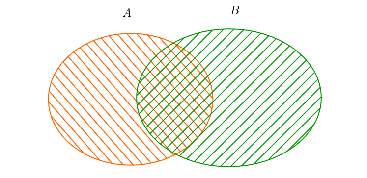
The second approach to define a set is to use another set(s). For example, if we have two sets \(A\) and \(B\), we can define their union, the set \(X\) as follows: \[ X \equiv A \cup B = \lbrace x \,|\, x \in A \lor x \in B \rbrace \] It may be read as: "A set \(X\) is a set of elements, where each element \(x\) belongs to \(A\) or belongs to \(B\)". In addition to the unions, there is the intersection: \[A \cap B\ = \lbrace x \,|\, x \in A \land x \in B \rbrace \]
and the difference: \[A \backslash B = \lbrace x\,|\, x \in A \land x \notin B \rbrace \]
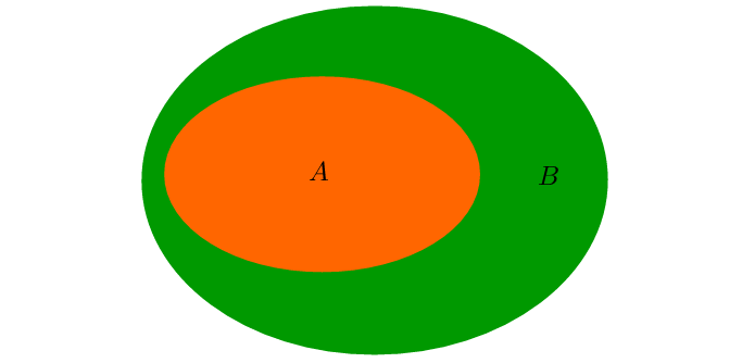
Also, between sets, like between all other mathematical entities of the same nature, there are different relations. For example, one set may be a part of another, in this case, we say "\(A\) is a subset of \(B\)" and write: \[A \subset B \Leftrightarrow A = \lbrace x\,|\, \forall x \in A \rightarrow x \in B \rbrace \]
Another important definition is the Cartesian product. If a set \(A\) and a set \(B\) have the same number of elements, then their "product" is also a set, containing the pairs of elements from both sets: \[ X = A \times B = \lbrace (x,y) \,|\, x \in A, y \in B \rbrace \] Similarly, the set exponentiation concept is introduced. For example, two-dimensional coordinate space: \[ \mathbb{R}^{2} \equiv \mathbb{R}\times\mathbb{R} = \lbrace (x,y) \,|\, x \in \mathbb{R}, y \in \mathbb{R} \rbrace \] Last important note regarding sets is that it is totally fine that some elements of a set may be infinite.
All this information about sets is useful to understand the next term: a mapping or a function. Let's discuss this briefly. There's a formal definition of a function:
Consider two sets \(X\) and \(Y\). Then, a mapping \(f\), defined on a set \(X\), is a rule, according to which, every element \(x\) of the set \(X\) is associated with some specific element \(y\) of the set \(Y\).
This fact may be denoted using the following notation: \(f: X \rightarrow Y\) or \(f: x \mapsto y\).
All elements function \(f\) is working with are called the domain and denoted by \(dom(f)\). Likewise, all possible elements \(y\) that can be obtained applying the function \(f\) make the codomain. The set of elements obtained by the action of the function on its domain is called the range, which is usually denoted as \(im(f)\). Now, for instance, we can formally define what a plain graph of the function \(f\) is. It is a set \(G(f) \subset X \times Y \): \[ G(f) = \lbrace (x, y) \, | \, x\in dom(f), \,\, y = f(x) \rbrace \] Also, a few more terms will be widely used further. Consider a subset \(A \subset dom(f)\), then the set \(f(A)\) is called the "image of \(A\) under \(f\)": \[ f(A) = \lbrace y \in Y \, | \, \exists x \in A \,\, y = f(x) \rbrace \] If we have two functions \(f: X \rightarrow Y\), \(g: im(f) \rightarrow Z\) and \(im(f) \subset Y\). Then, a function \(f \circ g : X \rightarrow Z\) is called the composition of these two functions. So, the composition is defined by the following rule: \(z = (f \circ g)(x) = g(f(x)), \, x \in X, \, z \in Z \).
In practice, we have to deal with a wide variety of functions. However, despite all functions are different (domain, range, their nature, and so on) they can be grouped into three major classes depending on their behavior:
- Surjective (many-to-one). The function \(f\) is surjective, then: \(\forall y \in Y, \, \exists x \in X \, : \, y = f(x) \). In other words for every element from the range, there's some corresponding domain element. A simple example is a parabola: \(y = x^{2}\) where for \(y=4\) there are two respective values: \(x= \pm 2\).
- Injective (one-to-one). In that case \(\forall a \in X, \, \forall b \in X \, : \, f(a) = f(b) \rightarrow x = y \). This means that \(y\) can't have many \(x\): different elements of the set \(X\) are mapped to the different elements of \(Y\). For example \(y=e^{x}\), because there is no real value maps to a negative number, although the opposite is correct.
- Bijective. Function \(f\) is bijective if and only if it is injective and surjective simultaneously: \(\forall a \in X, \, \forall b \in X \, : \, a \neq b \rightarrow f(a) \neq f(b) \land \forall y \in Y, \, \exists x \in X \, : \, f(x) = y \). In other words such function \(f\) is a one-to-one correspondence: each \(x\) is paired with exactly one \(y\), and vice versa, each \(y\) is paired with exactly one \(x\). The simplest example is a linear function: \(y=x\)
If, for example, our function \(f\) is bijective, then for some set \(B \subset im(f)\) there's defined an "inverse image of a set \(B\) under the inverse function \(f^{-1} : im(f) \rightarrow X \)":
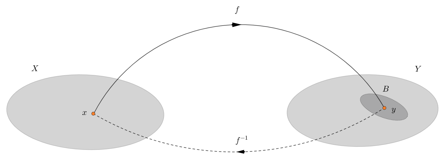
Thus, the inverse function just maps all \(y \in im(f)\) back to \(x \in dom(f)\). All other details regarding the functions will be described as we move forward.
Numbers
Now, when we've just remembered what the functions are, we can stop for a bit. And think about the things functions are working with. As we have already figured out, a function is a rule of mapping something from one set into something from the other set. This something may be anything: ranging from a mapping of some state's citizens last names to their driver license IDs to the simple linear function \(y = x\) that "transfers" numbers into themselves. To tell the truth, despite the fact that mathematics, in general, studies the behavior of abstract objects and the relations between them, it is the calculus that is mainly based on the fact that the objects under study are numbers. Whether it is integers, natural or real numbers - this is not that important.
Usually, the real numbers are used, like \( -1.75, 0, 2, 123.321\), and so on. The set of all real numbers is denoted by a special sign \( \mathbb{R}\), which already mentioned above. Despite an apparent simplicity, there's a specific field called number theory that studies all number-related questions and strictly introduce the definition of a real number. Here, we certainly don't need such a severity, so for our current needs, we can assume that the real numbers are the numbers, which may be used to measure any possible distance between two points on an infinitely long number line.
One essential thing we need to know about the real numbers is that "the space of real numbers is complete"3. What does that mean? Of course, intuitively, we can think about this as about an ability to measure any possible distance. There's a more strict equivalent of this thought called the Dedekind's theorem:
Assume \(A\) and \(B\) are some nonempty sets in \(\mathbb{R}\) with the following properties: \(\forall a \in A \,\, \forall b \in B \,\, a \le b\). Then \(\exists c \in \mathbb{R} \, | \, \forall a \in A \,\, \forall b \in B \,\, a \le c \le b\).
Or in other words, for any two numbers from \( \mathbb{R}\) there's a number between them:
Why are we even talking about this? Because this property is crucial for all our further considerations. Actually, all the next statements will be based on this fact either explicitly or implicitly. It is tricky to prove it. However, the Dedekind's theorem evidence is based on the intuitively-simple nested intervals theorem. So, we can assume that the completeness of \( \mathbb{R}\) is an axiom. So, it is time to go on further.
Infima and Suprema
The actual state of affairs does not give us an opportunity to move forward directly to derivatives - the first milestone of this series of posts. That being the case, we need to end up with functions. In order to do that, it is important to deal with sequences because their properties are the key to understanding the nature of functions.
Firstly, we need to define what the infimum and supremum are. Assume \(A \subset \mathbb{R}\), then a number \(u \in \mathbb{R}\) is an upper bound of the set \(A\) if \(\forall x \in a \,\, x \le u\). Likewise, then a number \(l \in \mathbb{R}\) is a lower bound of the set \(A\) if \(\forall x \in a \,\, l \le x\). Using these terms, we can define a bounded set. A set \(A \subset \mathbb{R}\) is bounded from above (below) if and only if there's at least one upper (lower) bound of the set \(A\). Thus, the set \(A\) is called bounded when it is bounded both from above and below. One important note: upper or lower bound are not obliged to be an element of the set they bound. Also, it is important not to confuse the term bound and the maximum or minimum of a set. There are maybe many bounds but only one maximum, if it exists, of course. For example, for the interval \((1,\,2)\), there is an infinite number of bounds, \(2, \, 3, \, ...\) but there is no maximum element at all.
Let's come back to our set \(A\) and consider it bounded from the above (below). Among the all existing upper (lower) bounds, there is a smallest (largest) one (like for any other set from \(\mathbb{R}\)). This least (greatest) value is called the supremum (infimum). Supremum and infimum are denoted as follows: \(\sup A\) and \(\inf A\) respectively. For example, the closed interval \([3, 5]\) has and infimum \(3\), and supremum \(5\).
The existence of suprema and infima is guaranteed by the completeness of \(\mathbb{R}\):
Every nonempty set of real numbers that is bounded from above has a supremum, and every nonempty set of real numbers that is bounded from below has an infimum.
This theorem is the basis for a lot of significant results obtained by calculus.
Limits of Sequences and Functions
To start with, I'd like to remind what a sequence is. Formally, "a sequence is a function defined on the set of natural numbers \(\mathbb{N}\)". Hence, a sequence is just a mapping rule: \(x_{n} \, : \, \mathbb{N} \rightarrow \mathbb{R}\). Historically, the entire sequence and its \(n\)-th element as well are denoted by the same notation: \(x_{n}\). It is worth to note, that in the definition, there is nothing said about the number of elements in a sequence: there are maybe two or infinite elements.
Among the variety of different sequences, there are those, which have the limit. Limit of a sequence is a number \(l \in \mathbb{R}\) that is defined by the following rule: \[ \forall \varepsilon > 0, \,\, \exists n_{0}(\varepsilon) \in \mathbb{N}, \,\, \forall n \ge n_{0}(\varepsilon) \rightarrow |x_{n} - l| < \varepsilon \] Well, first things first, how to read it?
A sequence \(x_{n}\) converges to \(l\) if and only if for any positive number \(\varepsilon\) there exists an integer \(n_{0}\) depending on \(\varepsilon\) such that, for all elements \(x_{n}\) with a sequence number \(n \ge n_{0}\), the absolute difference between \(x_{n}\) and \(l\) is less then \(\varepsilon\).
Any student of mathematics can repeat this definition, even if you try to wake this person up at night. This pretty long definition might be written, using the next brief notation: \(x_{n} \rightarrow a\) or \(\lim{x_{n}} = a\). Usually, people say that a sequence converges to some number or that the sequence has a limit. Sometimes these symbols are used with an additional annotation: \(n \rightarrow \infty\).
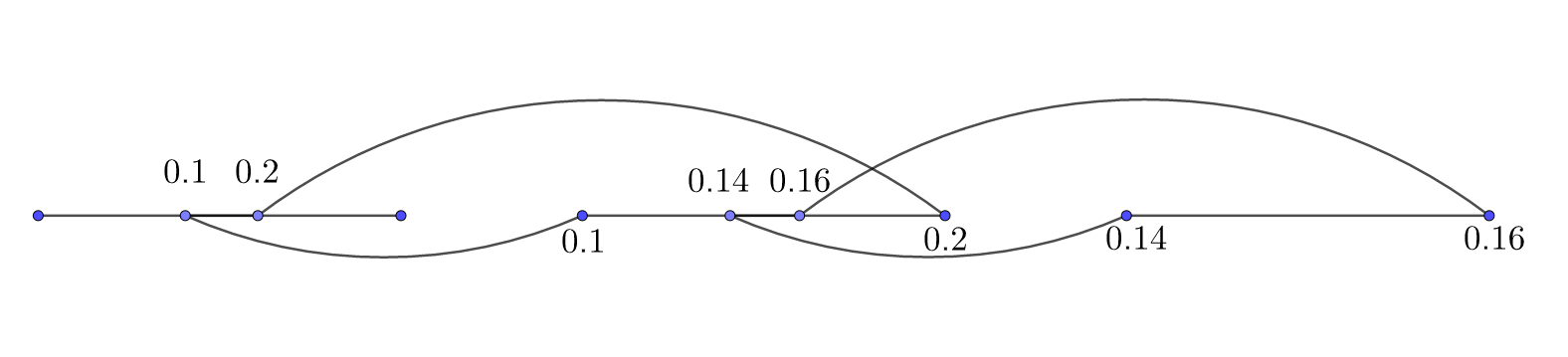
Let's take a look at the next example: sequence \(x_{n}=1+\sin (n) / n \) with a limit \(\lim{x_{n}} = 1\). The figure below illustrates how for some \(\varepsilon = 0.8\) the particular \(n_{0}=12\) might be found:
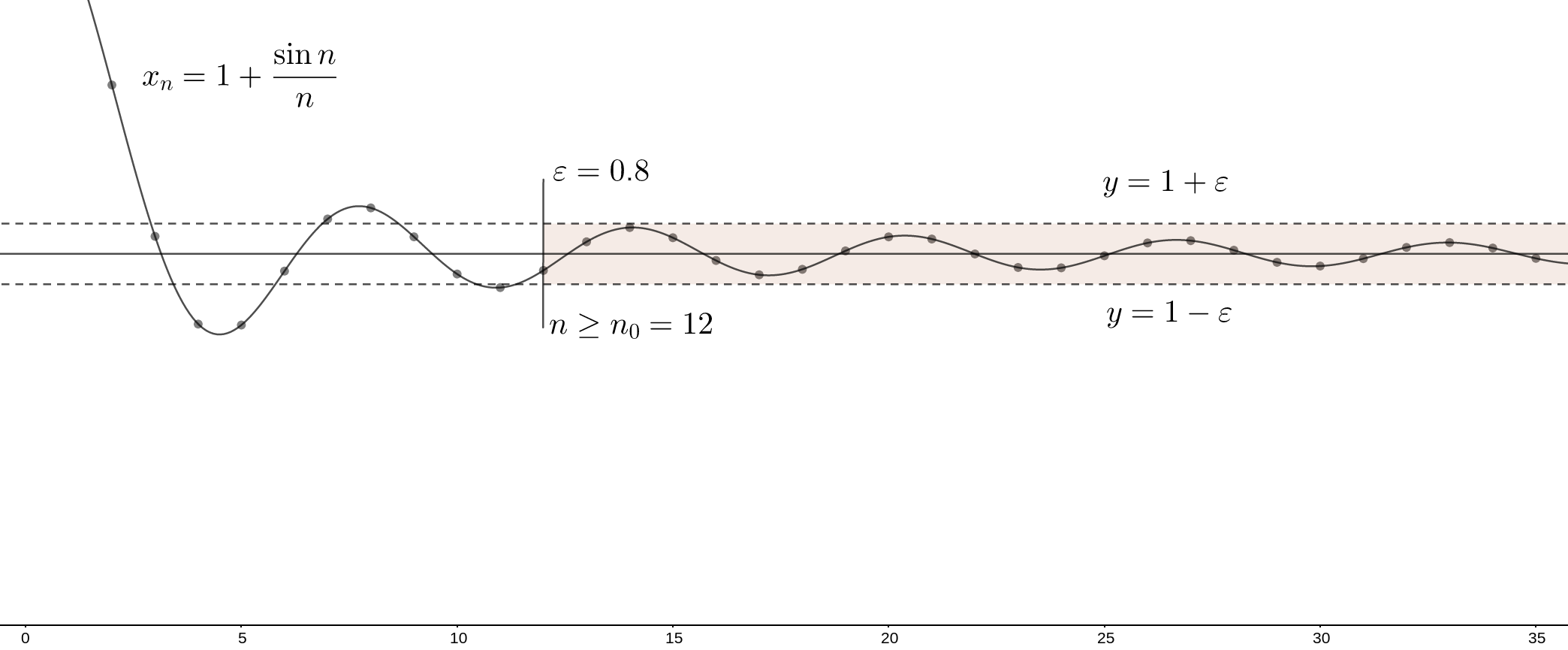
You can check, that for this case, we can empirically determine the function \(n_{0} = n_{0}(\varepsilon)\) from the definition above. Here, for instance, the following function works well: \(n_{0} = \dfrac{12 \cdot \ln (\varepsilon / 2)}{\ln (0.4)}\). By the way, such an approach of looking for some \(n_{0} = n_{0}(\varepsilon)\) along with the so-called Cauchy's convergence test, are the most popular methods used for the limits proofs.
Not any sequence necessarily has a limit. A good example is \(x_{n} = \sin (n) \) or \(x_{n} = (-1)^{n}\). Also, some sequences, like \(x_{n} = n\) for example, may have infinite limits: \[ \lim_{n\to\infty} x_{n} = \infty \Leftrightarrow \forall E > 0, \,\, \exists n_{0}(E) \in \mathbb{N}: \,\, \forall n \ge n_{0}(E) \rightarrow |x_{n}| > E \] For such cases, the word "tends" is used instead of "converges". There is a couple of theorems relating to the sequences, which are used for the proofs of some important facts, describing the nature of functions. Perhaps, the most frequently used one is the Bolzano–Weierstrass theorem that states, that any bounded sequence has a convergent subsequence.
Now, let's talk about the result of everything we discussed above: limit of functions. For convenience, limits are usually considered in the so-called limit (or accumulation) points:
A point \(a \in \mathbb{R}\) is a limit point of a set \(X \subset \mathbb{R}\), if \(X\) has points indefinitely close to the point \(a\) other than \(a\): \[ \forall \varepsilon > 0, \,\, \exists x \in X: \,\, 0 < |x - a | < \varepsilon \]
There are two more types of limit points: right or left limit points, where for a given point \(a\), there exist some points only from the left or right respectively. So, consider \(f \, : \, X \rightarrow \mathbb{R}, \, X \subset \mathbb{R}\) and \(a \in X\) is a limit point, then \(l \in \mathbb{R}\) is a limit of \(f(x)\) at \(a\): \[ \lim_{x\to a} f(x) = l \Leftrightarrow \forall \varepsilon > 0, \,\, \exists \delta(\varepsilon) > 0, \,\, \forall x \in X: \,\, 0 < |x - a| < \delta(\varepsilon) \rightarrow |f(x) - l| < \varepsilon \] Another way of writing this is: \(f(x) \xrightarrow[x \to a ]{} l \). This can be read as follows: function \(f\) has a limit \(l\) at a point \(a\), if and only if, for any positive \(\varepsilon\), it is possible to find some positive \(\delta\), that any point from \(l\)'s \(\varepsilon\)-neighborhood can be mapped into the punctured \(\delta\)-neighborhood of the point \(a\):
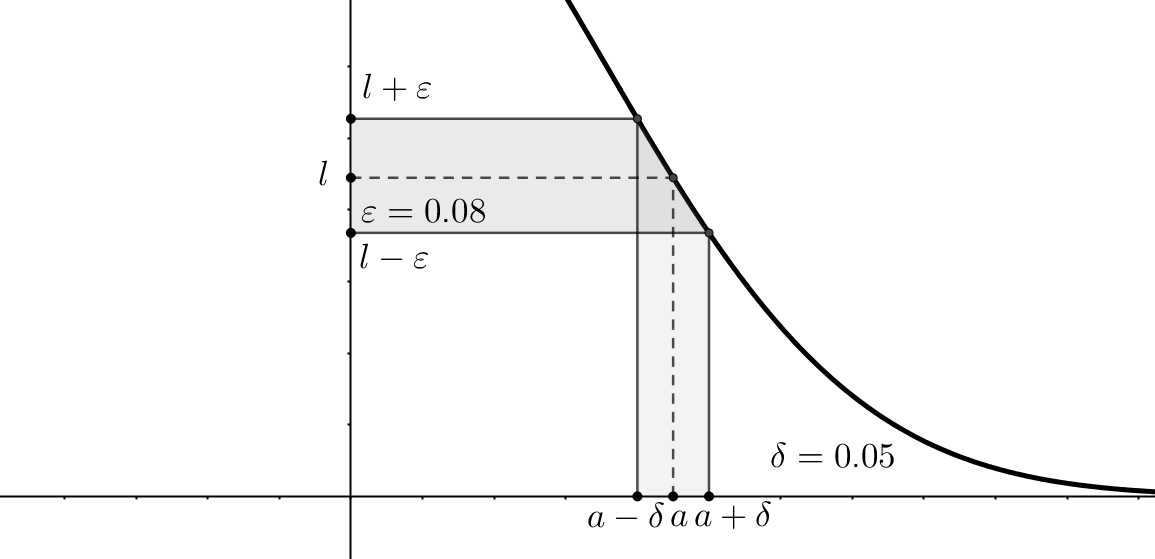
That is why it is denoted that \(\delta\) depends on \(\varepsilon\): \(\delta = \delta(\varepsilon)\). Exclusion of the limit point from the consideration is an important nuance, because the function value can be undefined at this point, for example, due to the division by zero.
In general, not every function has a limit at each point of its domain. Actually, assuming \(f \, : \, \mathbb{R} \rightarrow \mathbb{R}\) and some limit point \(a \in \mathbb{R}\) (\(a\) can also be \(+\infty\) or \(-\infty\)), there are several scenarios:
Sometimes functions have different limit's value at one point. Everything depends on the direction in which we approach that point4. If a function has different values on different sides of the same point, then it undergoes a discontinuity at it. Thus, when one-sided limits have different values, the regular double-sided limit defined above doesn't exist at this point:
The way how limits behave in the function composition case is pretty straightforward:
Consider a function composition \(g \circ f \, : \, X \rightarrow \mathbb{R}\, | \, (g\circ f)(x) = g(f(x))\), where \(f\, : \, X \rightarrow \mathbb{R}\), \(g\, : \, Y \rightarrow \mathbb{R}\) and \(f(X) \subset Y\). If there exist both \(\lim_{x\to a} f(x) = l_{1} \in \mathbb{R}\) and \(\lim_{y\to l_{1}} g(y) = l_{2} \in \mathbb{R}\), and for every \(x\in X \, | \, x \ne a \rightarrow f(x) \ne l_{1}\). Then there exists a limit of the composition \(\lim_{x\to a} g(f(x)) = l_{2}\).
Despite first glance transparency, this theorem, by the way, is frequently implicitly used in mathematical analysis proofs.
The last but not the least issue with limits of functions I would like to address relates to the way how usually the limit existence fact is being checked. Often, the original definition is used to check that the limit exists. However, sometimes it's needed to prove that at some point there's no limit. Such a fact can be proved using the so-called Cauchy criterion (which, by the way, was already mentioned above for sequences) that states that \(\lim_{x\to a} f(x) = l\) if and only if: \[ \underbrace{\forall \varepsilon > 0, \,\, \exists \delta > 0, \,\, \forall x_{1},x_{2} \in X}_{P}: \,\, \underbrace{0 < |x_{1} - a| < \delta, 0 < |x_{2} - a| < \delta}_{A} \rightarrow \underbrace{|f(x_{1}) - f(x_{2})| < \varepsilon}_{B} \] And it literally means, that the limit exists if and only if, for any two points close to \(a\) their mappings, to some extent, are close as well. \(\delta\) in this definition, of course, depends on the \(\varepsilon\) alike in the similar statements above and below.
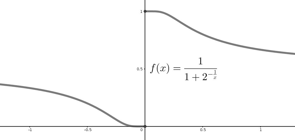
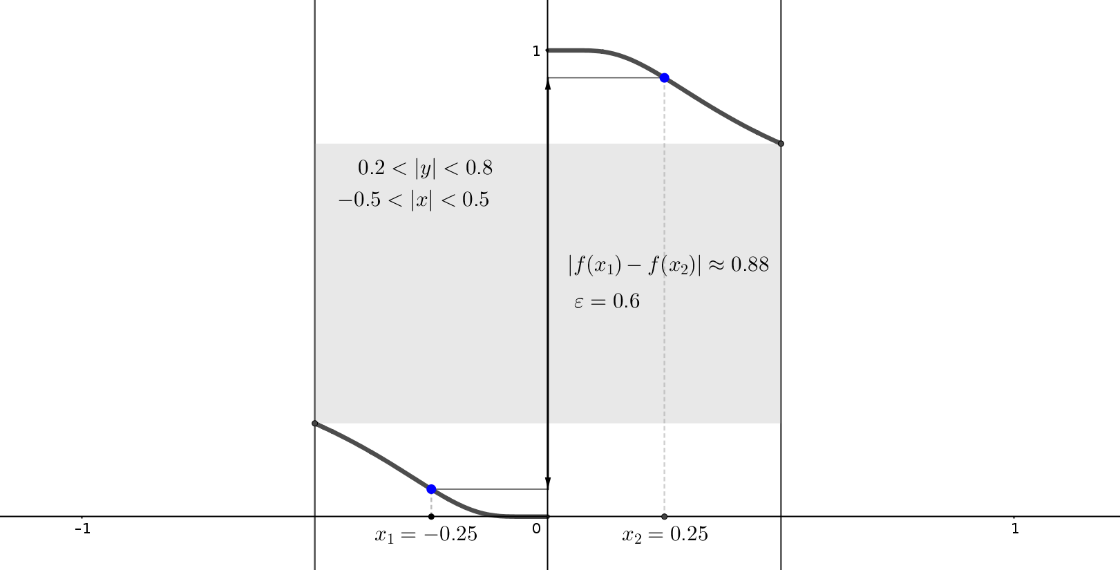
Let's prove that, for example, that the function in the figure above \(f(x) = (1 + 2^{-1/x})^{-1}\) has no limit at point \(x = 0\). In this case, we can negate the Cauchy criterion, i.e., if the criterion isn't satisfied then the limit doesn't exist. As stated in the statements and quantifiers section abvoe, during the negation, quantifiers are replaced with the opposite ones, and the implication \(A \rightarrow B\) is replaced with \(A \land (\lnot B) \). Finally, we get: \[ \underbrace{\exists \varepsilon > 0, \,\, \forall \delta > 0, \,\, \exists x_{1},x_{2} \in X}_{\lnot P}:\,\, \underbrace{0 < |x_{1} - a| < \delta, 0 < |x_{2} - a| < \delta}_{A} \land \underbrace{|f(x_{1}) - f(x_{2})| \ge \varepsilon}_{\lnot B} \] This expression states, that there exists some positive \(\varepsilon\), that for any positive \(\delta\), there are two points \(x_{1},x_{2}\) inside \(a\)'s \(\delta\)-neighborhood, whose \(f(x_{1})\) and \(f(x_{2})\) aren't close. In our example, not strictly speaking, we can consider, for instance, \(\varepsilon=0.6\) and, as you can see, for whatever \(\delta\) you'll chose (for example \(\delta=0.5\)), you can find such two points inside zero's \(\delta\)-neighborhood. For example, if \(x_{1}=-0.25\) and \(x_{2}=0.25\), then \(|f(x_{1})-f(x_{2}| \approx 0.88 \ge \varepsilon = 0.6\) is true. This proves that \(f\) has no limit at \(x = 0\):
By the way, some functions have pretty surprising values of the limits at their special points. Here are the two most famous examples:
Continuity
Great, we are almost done! Let's take a look at the probably one of the key concepts the whole calculus is based on. Why is continuity so important? It is because most of the functions which are used in physics, math, at last in machine learning are changing smoothly, without "fractures", in other words, such functions are continuous. If a function is discontinuous, we cannot calculate its derivative or integral as well as to approximate it with simple functions, using, for example, Taylor or Fourier series. This is why this property is fundamental in calculus. So, to be more precise:
A function \(f \, : \, X \rightarrow \mathbb{R}\) is called continuous at a point \(a\in X\) if: \[ \forall \varepsilon > 0, \,\, \exists \delta(\varepsilon) > 0, \,\, \forall x \in X: \,\, |x - a| < \delta(\varepsilon) \rightarrow |f(x) - f(a)| < \varepsilon \]
If we compare this definition to the function limit's definition given above, we can see, that in the case when a point \(a\) is the limit point of \(f\), the continuity simply means equality of the function value to its limit at a given point: \(\lim_{x\rightarrow a} f(x) = f(a)\) - that is how the continuity-at-a-point property is tested in practice.
Also, sometimes it is convenient to consider continuity in the terms of function increments. Let me remind, that increment of a function \(f(x)\) at a point \(x\), that is close to the point \(x_{0}\), is called the difference \(\Delta f = f(x) - f(x_{0})\). Or, using the argument increment \(\Delta x = x - x_{0}\), the above expression can be written as follows: \(\Delta f = f(x_{0}+\Delta x) - f(x_{0})\). Thus, in accordance with the continuity definition through the limit, we have, that a function \(f(x)\) is continuous at a point \(x_{0}\) if and only if \(\lim_{\Delta x\rightarrow 0} \Delta f = 0\).
For example, let's prove that the function \(f(x)=x^{3}-x+1\) is continuous everywhere on its domain \(\mathbb{R}\): \[ \Delta f = (x_{0}+\Delta x)^{3}-(x_{0}+\Delta x)-1-x_{0}^{3}+x_{0}-1 = {\Delta x}^{3} + 3 x^{2} \Delta x + 3x {\Delta x}^{2}-\Delta x = \] \[ = \Delta x \cdot ({\Delta x}^{2}+3x\Delta x + 3x^{2}-1) \xrightarrow[\Delta x \to 0 ]{} 0 \,\, \forall x \in \mathbb{R} \,\, \quad \blacksquare \] Here, as you can see, this trick helps to "extend" the study area on the entire domain, thereby simplifying the process quite significantly.
The property of continuity extends to compositions of two continuous functions, such as their addition, subtraction, multiplication, and division. If a function is discontinuous at some point, then this discontinuity might be classified as removable, jump or essential discontinuity. The last type of discontinuity is an extremely important topic of complex analysis.
The continuity of a function on the closed interval, as already mentioned, is an incredibly strong property. For example, it provides the basis for the presence of the function's maximum and minimum (extreme value theorem), as well as the presence of an inverse function defined on this interval (inverse function theorem).
...
I hope that this post turned out to be helpful to freshen up your knowledge and now, we can move forward. In the next post, we will proceed to the next step - derivatives.
References
It is a list of basic mathematical analysis (and not only) books I found useful to write this and the follow-up posts:
- Jim Hefferon - "Linear Algebra". Illustrated course to the basics of linear algebra with many examples. Link.
- John E. Hutchinson - "Introduction To Mathematical Analysis". Short and clear mathematical analysis course from Australian National University. Link.
- Walter Rudin - "Principles of Mathematical Analysis". Collection of essential mathematical analysis theorems and their detailed proofs. Link.
- Thomson, Brian S., Judith B. Bruckner, and Andrew M. Bruckner - "Elementary real analysis". Well-structured guide to the real analysis with plenty of good and illustrative examples. Link.
Notes
- There is a nice Wikipedia page describing the history of mathematical notation. ↩
- See this course for more details. ↩
- The question of completeness of some spaces is studied in the course of functional analysis. Unfortunately, for now, this question is out of the scope of this post. ↩
- Sometimes, the limit exists only at one side.↩