Why Are Planet Orbits Elliptical?
Preface
If you are outside the city, find an opportunity to look at the sky at night. If you are lucky enough, the sky will be clear, and if the air is cold, you will see the Milky Way along with millions of sparkling stars covering the entire sky. You'll certainly remember that for a long time...
Most of us at least once in life, lying under the night sky have thought about space. Why are there so many stars? Why do they shine? Why do some of them have planets that rotate around them? So, finally, how does it all work together? I have always been interested in these questions, so I decided, even though along with my modest efforts, to try and make astronomy a little more popular among the masses.
Of course, neither in a blog like this one nor in any book, it is impossible to answer even some of the questions above. So this series of astronomical notes will cover some simple, I would even say, everyday astronomy topics. These cosmic questions will be touched upon mostly superficially, in a scientifically-popular style, but I will try to make it so that the “computations lovers”, too can find something interesting for themselves.
Astronomy
Before we start, I would like firstly to talk a bit about astronomy. Astronomy is a natural science that studies the motion, structure, origin, and evolution of celestial bodies and their systems. It is one of the most ancient sciences which emerged based on the practical necessities of humans and has always been developing along with them.
The first mentions of astronomy date back to ancient Egypt and China, where simple astronomical observations were being used for time and orientation measurements. Nowadays, astronomy is widely used for geographical positioning as well as precise time measurements. Astronomy helps study the Earth and space. For example, without astronomy today, there would be no taxi services and plenty of maps that we all are accustomed to use. Modern astronomy is closely connected with math and physics, and chemistry and geography. Astronomy, using the achievements of other sciences, enriches them and stimulates their development, giving them an increasing amount of new challenges.
What Is This Post About?
This post is written to touch on, perhaps, the most common question that people across the world have been asking since their childhood: “Why and how do planets rotate around the Sun?”. Let’s start with the fact that our Solar System consists of one central star - the Sun and 8 (previously 9 with Pluto) large planets. All these planets have different sizes, masses, chemical elements they are made of, orbital periods, and so on. However, they all are united by one essential fact: they rotate around the Sun by elliptical orbits. Let's figure this out. But before I start writing some formulas, you probably want to ask another question: "Why are we talking only about the Solar System? Is this rotation fact true only for it?". Answer is no. It is a universal phenomenon, which doesn't depend on place and can be applied both in small star systems with only one planet and for systems with many planets, like the Solar System we live in. Thus, we can consider the problem from the most general, mathematical point of view.
Moreover, I want to add that this post does not cover the question of why the Solar System's planets, at some point, started to rotate around the Sun, which is still a topic of hot discussions in the scientific community (there are different theories explaining that). So we will consider the planets' rotation as fact.
History
First of all, it is useful to have some historical context of the planet rotation problem. In the early XVII century, the famous German astronomer Johannes Kepler discovered laws under which the movement of satellites around the center of gravity takes place.
Kepler was engaged in the analysis of a large number of astronomical observations, which were already available by then. The data contained information about the Solar System's planet motion. Among the chaos of seemingly at first glance unrelated numbers, he managed to discern the beautiful and simple patterns: namely that, the orbits of the planets are elliptical1 and their parameters are interrelated. The latter is obvious, if only from the fact that all planets have a single center of attraction: the Sun. In Kepler's laws, nature once again discovers the rationality of its structure.
However, Kepler did not give any physical explanation for the laws he discovered. His work was more of a philosophical nature, which was the hallmark of any scientific research during that period. After the discovery of the laws of planetary motion, a little more than 50 years passed and the English physicist Isaac Newton gave them a robust physical-mathematical explanation. Moreover, incidentally, as an "application", he formulated the fundamental laws of mechanics as well as the law of universal gravitation, and developed the foundations of differential computation in his famous work - “Philosophiæ Naturalis Principia Mathematica.” Newton needed derivatives to overcome difficulties in describing the uneven motion (see this post about derivatives).
Now, we will attempt to reproduce a theoretical way to determine the laws of Kepler, for a little while, becoming participants of their "second discovery".
Kepler’s Motion
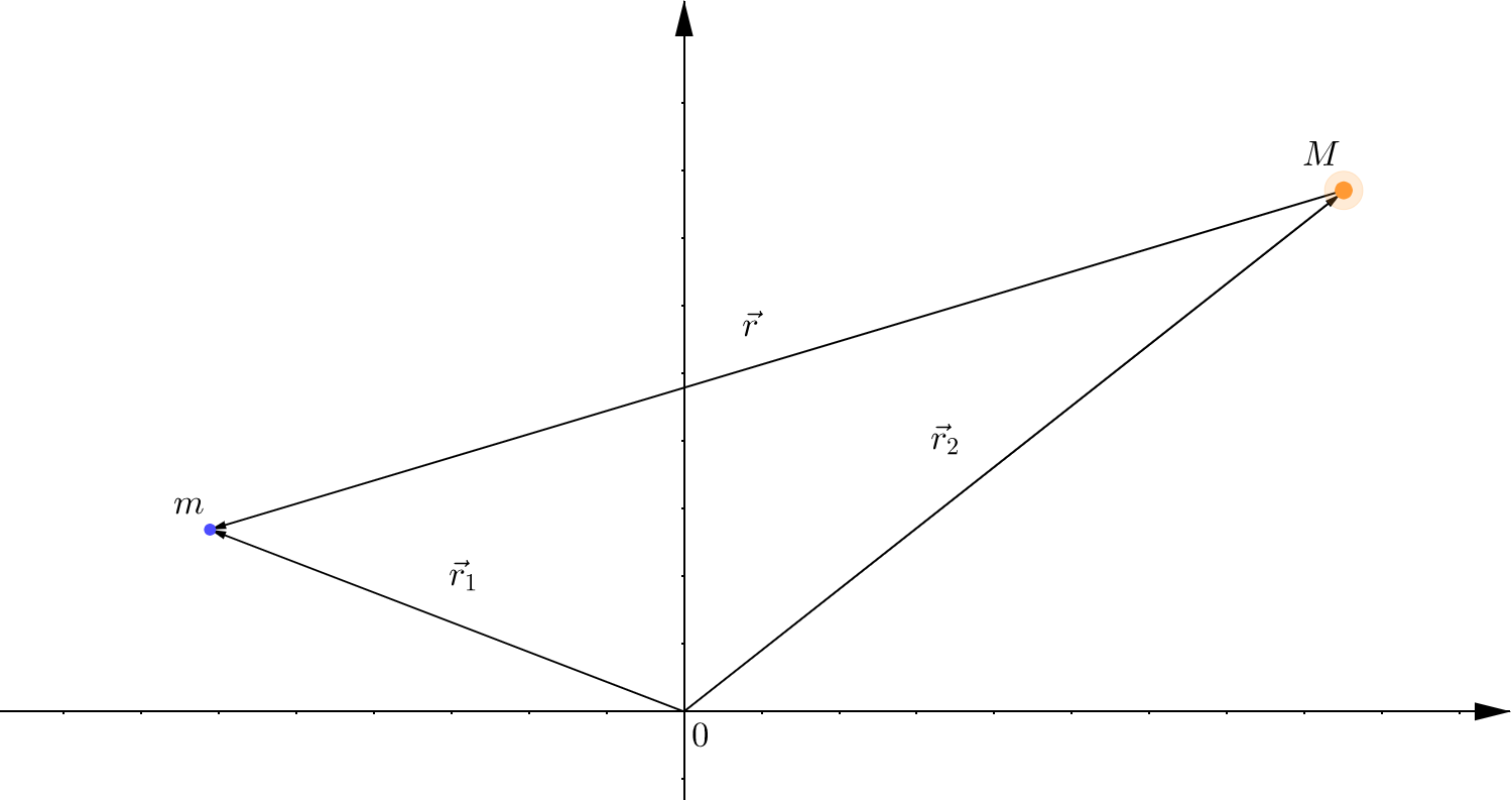
Let us consider the movement of some planet with mass \(m\) around the Sun with mass \(M\). Also, suppose \(\vec{r}_{1}\) and \(\vec{r}_{2}\) are their position vectors respectively, so \(\vec{r} = \vec{r}_{1} − \vec{r}_{2}\) is a distance between the planet and the Sun:
Since even for the heaviest planet, Jupiter, \(m/M \approx 1/2000\), the Sun with a very good precision might be assumed as motionless, and the mutual attraction between the planets can be disregarded in the leading-order term. Formally, if we want to write down Newton's second law of motion using the law of universal gravitation in a vector form, it will give us the following2:
\[\begin{equation}m \ddot{\vec{r}}_{1} = − \dfrac{GMm}{|\vec{r}|^{3}}\vec{r} \end{equation} \]
\[\begin{equation}M \ddot{\vec{r}}_{2} = \dfrac{GMm}{|\vec{r}|^{3}}\vec{r} \end{equation}\]
\[(1)/m + (2)/M \Rightarrow \ddot{\vec{r}} = − \dfrac{G(M + m)}{|\vec{r}|^{3}}\vec{r} \]
So, assuming \(M \gg m\), the given equation confirms our initial hypothesis that the Sun's motion may be omitted. Hence, under all assumptions made above, the motion of the planet around a static point-like gravitational center can be described using the following expression:
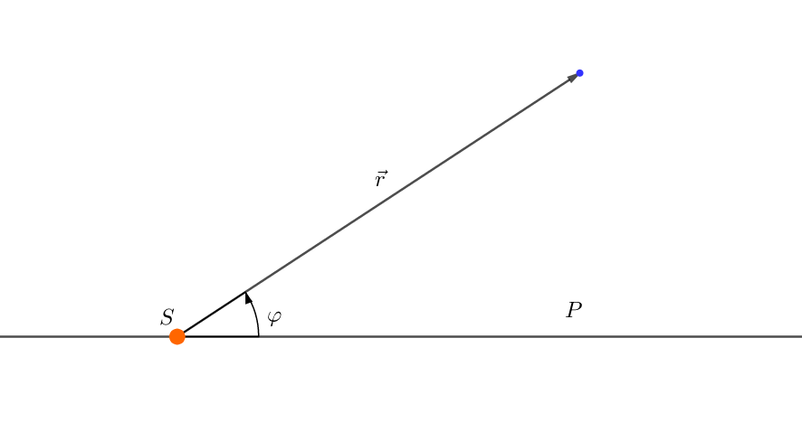
\[\begin{equation} \ddot{\vec{r}} = − \dfrac{GM}{|\vec{r}|^{3}}\vec{r} \end{equation}\]It's intuitively clear that during such motion, both the length \(r \equiv |\vec{r}|\)3 of position vector \(\vec{r}\) and its direction are being changed. The direction can be described by the polar angle \(\varphi\) between \(\vec{r}\) and some fixed direction \(SP\):
One wonders how we can use that to simplify \((3)\)? It turns out that it is not as difficult as it seems at first glance. All we need to do is take into account some geometric considerations. As stated above, it is more convenient to consider the motion in polar coordinates \((r, \varphi)\), which has two perpendicular basis vectors \(\vec{e}_{r}\) (along \(\vec{r}\)) and \(\vec{e}_{\varphi}\) (perpendicular to \(\vec{e}_{r}\)), so \(\vec{r} = r\vec{e}_{r}\).
\((3)\) uses the second derivative for \(\vec{r}\). In order to be able to represent it in a useful form, we need to establish a connection between how changes in polar vectors (the planet's actual moving) in time can be related to each other. Furthermore, everyone's favorite unit circle is the well-known "tool" that can help us out:
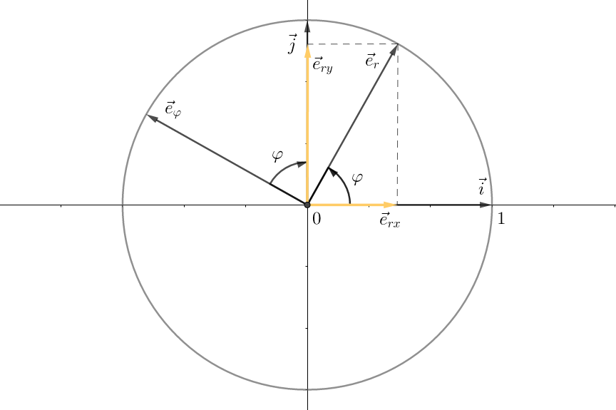
As it indicated in the above illustration, we can expand these two polar basis vectors using the Cartesian coordinate system basis vectors \(\vec{i}\) and \(\vec{j}\): \[ \vec{e}_{r} = \vec{e}_{rx} + \vec{e}_{ry} = \vec{i} \cdot \cos{\varphi} + \vec{j} \cdot \sin{\varphi}; \qquad \vec{e}_{\varphi} = −\vec{i} \cdot \sin{\varphi} + \vec{j} \cdot \cos{\varphi}\] It means that for constant \(\vec{i}\) and \(\vec{j}\) basis vectors, we get the following partial derivatives of \(\vec{e}_{r}\) and \(\vec{e}_{\varphi}\) with the respect to \(\varphi\)4: \[\begin{equation} \dfrac{\partial \vec{e}_{r}}{\partial\varphi} = \vec{i} \cdot \dfrac{d\cos{\varphi}}{d\varphi} + \vec{j} \cdot \dfrac{d\sin{\varphi}}{d\varphi} = −\vec{i} \cdot \sin{\varphi} + \vec{j} \cdot \cos{\varphi} = \vec{e}_{\varphi}\end{equation}\] \[\begin{equation} \dfrac{\partial \vec{e}_{\varphi}}{\partial\varphi} = −\vec{i} \cdot \dfrac{d\sin{\varphi}}{d\varphi} + \vec{j} \cdot \dfrac{d\cos{\varphi}}{d\varphi} = −\vec{i} \cdot \cos{\varphi} − \vec{j} \cdot \sin{\varphi} = − \vec{e}_{r} \end{equation}\] Perfect! Now, recalling the derivatives chain rule and the derivatives product rule, we can calculate \(\ddot{\vec{r}}\). So, firstly: \[\vec{v} \equiv \dot{\vec{r}} = \dfrac{d(r\cdot \vec{e}_{r})}{dt} = \dot{r}\vec{e}_{r} + r\dfrac{d\vec{e}_{r}}{dt} = \dot{r}\vec{e}_{r} + r\dfrac{\partial\vec{e}_{r}}{\partial\varphi}\dfrac{d\varphi}{dt} = \dot{r}\vec{e}_{r} + r\dot{\varphi}\vec{e}_{\varphi} \] , where \( v_{r} = |\vec{v}_{r}| = \dot{r}\) and \(v_{\tau} = |\vec{v}_{\tau}| = \omega =r\dot{\varphi}\) are radial and angular velocities respectively. Of course, it was possible to get an expression for \(\dot{\vec{r}}\) using purely physical considerations. However, for more clarity, I guess that aforementioned calculations might be pretty useful. Next, by doing the same and using equations \((4)\) and \((5)\), we have: \[\vec{a} \equiv \ddot{\vec{r}} = \dfrac{d\dot{\vec{r}}}{dt} = \dfrac{d}{dt} \left(\dot{r}\vec{e}_{r} + r\dot{\varphi}\vec{e}_{\varphi} \right) = (\ddot{r}\vec{e}_{r} + \dot{r}\dot{\varphi}\vec{e}_{\varphi}) + (-r\dot{\varphi}^{2}\vec{r}+\dot{r}\dot{\varphi}\vec{e}_{\varphi} + r\ddot{\varphi}\vec{e}_{\varphi}) = \] \[\begin{equation} = (\ddot{r}-r\dot{\varphi}^{2})\vec{e}_{r} + (2\dot{r}\dot{\varphi} + r\ddot{\varphi})\vec{e}_{\varphi} \end{equation}\] So finally, leveraging the fact that two vectors are equal if and only if their corresponding coordinates are equal, we can divide equation \((3)\) into two vector-independent ones. Thus, we've got two second-order differential equations for functions \(r=r(t)\), and \(\varphi=\varphi(r)\) which depend on time \(t\): \[\begin{equation} (3) \Leftrightarrow (\ddot{r}-r\dot{\varphi}^{2})\vec{e}_{r} + (2\dot{r}\dot{\varphi} + r\ddot{\varphi})\vec{e}_{\varphi} = -\dfrac{GM}{r^{3}}(r\vec{e}_{r} + 0\vec{e}_{\varphi}) \Leftrightarrow \begin{cases} \ddot{r}-r\dot{\varphi}^{2} = -\dfrac{GM}{r^{2}} \\ 2\dot{r}\dot{\varphi} + r\ddot{\varphi} = 0 \end{cases} \end{equation}\] We are halfway to the solution!
The Solution
Well, what should we do to solve the system \((7)\)? It is a very good question. However, this system contains products of functions and their derivatives, i.e., the equations are nonlinear. It is not a secret that solving nonlinear differential equations is much more complex than solving the linear ones. Moreover, the equations have second order terms, and the presence of two closely related functions \(r=r(t)\) and \(\varphi=\varphi(r)\) sufficiently complicates things. So what are we going to do?
The key to the solution is to take a look at the system \((7)\) from another point of view. Let's forget for a moment about the dependency of our functions from time and try to focus on the actual planet's trajectory: \(r=r(\varphi)\). In order to figure that out, we have to exclude \(t\) from the system. How? It is not that difficult: the only thing we have to do is just to recall the fact that every small change in time produces the change of the angle, or that, in other words, based on the chain rule, we have: \[ \dfrac{dr}{dt} \equiv \dfrac{d}{dt}(r(\varphi(t)) = \dfrac{\partial r}{\partial\varphi} \cdot \dfrac{\partial\varphi}{\partial t} \] Using this expression and assuming by default that all derivatives are actually partial, after transformation of the first and second equations in the system \((7)\): \[\ddot{r} = \dfrac{d}{dt} \left (\dfrac{d r}{d\varphi} \cdot \dfrac{d\varphi}{dt} \right ) = \dfrac{d}{dt}\left(\dfrac{dr}{d\varphi} \right) \cdot \dfrac{d\varphi}{dt} + \dfrac{dr}{d\varphi} \cdot \dfrac{d}{dt}\left(\dfrac{d\varphi}{dt} \right) = \dfrac{d}{d\varphi}\left(\dfrac{dr}{d\varphi}\right) \cdot \dfrac{d\varphi}{dt} \cdot \dfrac{d\varphi}{dt} + \] \[ + \dfrac{dr}{d\varphi} \cdot \dfrac{d^{2}\varphi}{dt^{2}} = \left(\dfrac{d\varphi}{dt} \right)^{2} \cdot \dfrac{d^{2}r}{d\varphi^{2}} + \dfrac{dr}{d\varphi}\cdot \dfrac{d^{2}\varphi}{dt^{2}} \Rightarrow \]
\[\begin{equation} (7) \Leftrightarrow \begin{cases} r_{\varphi\varphi} \dot{\varphi}^{2} + r_{\varphi}\ddot{\varphi}-r\dot{\varphi}^{2} = -\dfrac{GM}{r^{2}} \\ 2r_{\varphi}\dot{\varphi}^{2} + r\ddot{\varphi} = 0 \end{cases} \end{equation}\]Unfortunately, here, we see again that \((8)\) still contains time as an explicit variable. Therefore, we need to find out some additional considerations. Let's try and think back to the original task and consider the way how the gravitational force acts on our planet:
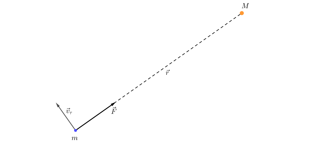
Since the gravitational force is central force, i.e., it is directed along the position vector \(\vec{r}\), we can use the conservation of the angular momentum law. Alternatively, more formally, assuming that \(L\) is an initial value of the planet's angular momentum: \[ \vec{r} \uparrow\uparrow \vec{F} \Leftrightarrow \vec{r} \times \vec{F} = 0; \, \vec{r} \times \vec{F} = \dfrac{d}{dt}\left(\vec{r} \times \vec{p}\right) = \dfrac{d\vec{L}}{dt} \Rightarrow \dfrac{d\vec{L}}{dt} = 0 \Rightarrow |\vec{L}| = \text{const} = L \] On the other hand, initial momentum can be calculated using the expression for the planet's angular velocity \(v_{\tau} = r\dot{\varphi}\): \[\begin{equation} L = | \vec{r} \times \vec{p} | = mr \cdot |\vec{v}_{\tau}| = mr^{2} \cdot \dot{\varphi} \Rightarrow \dot{\varphi} = \dfrac{L}{mr^{2}} \end{equation}\] Now we know how the angle changes are connected with the distance \(\vec{r}\). Perfect! This is the last piece of the puzzle! By the way, there's one more detail related to the equation we just got. For a small amount of time \(dt\), the planet sweeps out a small triangle with an area that equals to: \[ dS = \dfrac{1}{2}r\cdot(r + dr)\cdot\sin{d\varphi} \approx \dfrac{1}{2}r^{2}d\varphi \] So, \(dS/dt \propto L/m = \text{const}\). This equation is known as Kepler's Second Law, which will help us continue solving the system \((8)\).
Now, we need to exclude the derivative \(\ddot{\varphi}\) from the first equation of the system \((8)\) using the expression \((9)\) to substitute \(\dot{\varphi}\): \[ \left(\dfrac{L}{mr^{2}}\right)^{2} \cdot (r_{\varphi\varphi} - r) + \left[-\dfrac{2}{r} \cdot r_{\varphi} \left(\dfrac{L}{mr^{2}}\right)^{2} \right]\cdot r_{\varphi}= -\dfrac{GM}{r^{2}} \Leftrightarrow \] \[\begin{equation} \Leftrightarrow r_{\varphi\varphi} - \dfrac{2}{r}r_{\varphi}^{2} - r = -\dfrac{GM(mr)^{2}}{L^{2}} \end{equation}\] That's exactly what we wanted: an equation whose solution is the desired trajectory \(r(\varphi)\). This equation is non-linear, has the second order and it just cannot be easily integrated. Everything is not that simple... but there's a trick! Let's see if we can use the variable substitution approach here. We can try out the following substitution: \(u(\varphi) = 1 / r(\varphi)\), then: \[ r_{\varphi} = \dfrac{d}{d\varphi}\left(\dfrac{1}{u}\right) = -\dfrac{1}{u^{2}}u_{\varphi}; r_{\varphi\varphi} = \dfrac{d}{d\varphi}\left(-\dfrac{1}{u^{2}}u_{\varphi}\right) = \dfrac{2}{u^{3}}u_{\varphi}^{2} - \dfrac{1}{u^{2}}u_{\varphi\varphi} \] Plugging it into \((10)\) yields: \[ \dfrac{2}{u^{3}}u_{\varphi}^{2} - \dfrac{1}{u^{2}}u_{\varphi\varphi} - 2u\left(-\dfrac{1}{u^{2}}u_{\varphi}\right)^{2} - \dfrac{1}{u} + \dfrac{GMm^{2}}{L^{2}}\dfrac{1}{u} = 0 \] Do you see that?! Lo and behold! The terms with \(u_{\varphi}^{2}\) have been canceled out, giving: \[ \dfrac{d^{2}u}{d{\varphi}^{2}} + u = \dfrac{GMm^{2}}{L^{2}} \] It's a well-known heterogeneous harmonic oscillator equation and its general solution looks as follows: \[ u(\varphi) = \dfrac{GMm^{2}}{L^{2}} + C_{1} \cdot \cos(\varphi + C_{2}) \] Lastly, coming back to the planet's trajectory \(r(\varphi)\), let's define more convenient constants \(A \equiv C_{1}\) and \(-\varphi_{0} \equiv C_{2}\): \[\begin{equation} r(\varphi) = \dfrac{1}{(GMm^{2}/L^{2}) + A \cos(\varphi-\varphi_{0})} \equiv \dfrac{p}{1 + e \cdot \cos(\varphi-\varphi_{0})}, \end{equation}\] where, by the definition: \[ p = \dfrac{L^{2}}{GMm^{2}}, \quad e = A \cdot \dfrac{L^{2}}{GMm^{2}} \] Here, \(e\) is not Euler's number \(2.71...\) but it is the so-called eccentricity and \(p\) is the semi-latus rectum or the focal parameter. And if \(0 < e < 1\), we get, yes, the equation of the ellipse!
We have just accomplished our goal! We have proven that under certain conditions, planets are rotated around their stars by elliptical orbits. We only need to determine these conditions. Don't worry, it is much easier than what we have already done above. It's required to recall the energy conservation law and use some geometrical properties of an ellipse.
Let's count the angle \(\varphi\) in terms of when the planet is at the closest point to the Sun (\(r_{p}\) - the perigee), then \(\varphi = 0\) and respectively, in the most distant point (\(r_{a}\) the apogee) \(\varphi = \pi\), in that case \(\varphi_{0} = 0\). Thus, \[ r_{p} = \dfrac{1}{1 + e}, \quad r_{a} = \dfrac{1}{1 - e} \] So, if our planet has velocity \(v_{a}\) and \(v_{p}\) in the apogee and the perigee respectively, the energy conservation law may be written as follows: \[ E = \dfrac{m{v_{a}}^2}{2} - \dfrac{GMm}{r_{a}} = \dfrac{m{v_{p}}^2}{2} - \dfrac{GMm}{r_{p}} = \text{const} \] Of course, the angular momentum is preserved as well: \[L = mv_{a}r_{a} = mv_{p}r_{p} = \text{const} \] I don't want to bore you with the details, and I hope you can understand the same easily. So, combining these two equations together, and using \(p\) from \((11)\), we have: \[e = \sqrt{1 + 2mE\left(\dfrac{L}{GMm^{2}}\right)^{2}}\] Thus, finally, the aforementioned curve's parameters are entirely determined by the initial planet-and-the-Sun system's energy \(E\), its angular momentum \(L\), and their masses.
Analyzing the given expression for \(e\), in order to get an elliptical orbit, we need to impose the following constraints: \(0 \le e < 1\). This is possible if and only if: \[-\dfrac{1}{2m}\left(\dfrac{GMm^{2}}{L}\right)^{2} \le E < 0\] And if \(e = 0\), then the planet would move along the circular trajectory.
In total, the limited motion is possible only with negative energy: \(E < 0\)5. Using the expression for the planet's energy, we can reformulate this condition: \[E < 0 \Leftrightarrow v_{a} < \sqrt{\dfrac{2GM}{r_{a}}} \]
This condition is known as the escape velocity. Moreover, elementary math shows that for the Earth-Sun system escape velocity is about \(42 km/s\). However, the Earth's orbital speed is close to \(29 km/s\), Therefore, as you've already noticed, this condition is satisfied. Likewise, it is not hard to check that the expression above is true for all other planets in the Solar System.
Moreover, if \(E = 0\), then \(e = 1\) and, consequently, the planet will be moving along the parabolic trajectory. In this case, of course, such an object could not have been a planet. Therefore, this is most likely an interstellar object. Lastly, in the case when \(E > 0\), \(e > 1\), then the object will be moving along the hyperbolic trajectory.
Congratulations! Today, we theoretically got the laws experimentally established by Kepler and mathematically figured out by Newton. Thus, we finally determined all the terms under which a planet will be moving along the limited trajectory: an ellipse.
Notes
- There is a very informative Wikipedia page describing an ellipse. ↩
- A dot above a symbol means the derivative with respect to time. ↩
- For brevity, all vectors without the arrow signs mean their length. ↩
- The partial derivative symbol \(\partial\) is used to highlight that the functions, which are used for some particular derivative calculation, depend only on the single corresponding variable. See this post about derivatives as well as these and these Wikipedia notes. ↩
- Don't be afraid of negative energy values. Energy is a relative measure of the interaction between bodies. In our case, it is the gravitational force, and its field is the conservative force field with a potential considered negative only for convenience. You can read more about it here ↩