Multilayer Perceptron.
Part I: Introduction.
Today I would like to continue recently started conversation about machine learning and give more details on how the conventional architecture, called a multilayer perceptron, works. This post will contain information about the basic concepts used in, let's name it, neural networks theory.
Unlike the previous post, this and the subsequent ones, in addition to the general notes, contain some formulas, thus the one who likes mathematical strictness, I hope, will find something interesting as well. How can that be useful? First, it can be useful to those, who work in the field of machine learning or to those, who are simply interested in it. Also, in my opinion, it is tough to obtain a beneficial result in practice without an understanding of the basics: how things work from the inside. Secondly, generally speaking, neural networks in a large variety of their different architectures have a lot in common. Also, it is the perceptron that is the very foundation, the awareness of which will help greatly simplify further immersion in the world of neural networks and advanced ML technologies.
For a complete understanding of cause-effect relationships, before reading the text below, I would like to ask you to refresh your knowledge in probability theory, mathematical statistics, linear algebra, and calculus.
The multilayer perceptron will be mostly used as an example, but many of the conclusions that we will make are valid for many other ML algorithms.
Machine Learning Methods
Firstly, let me remind you that most of the machine learning methods can be categorized into two branches: supervised and unsupervised learning.
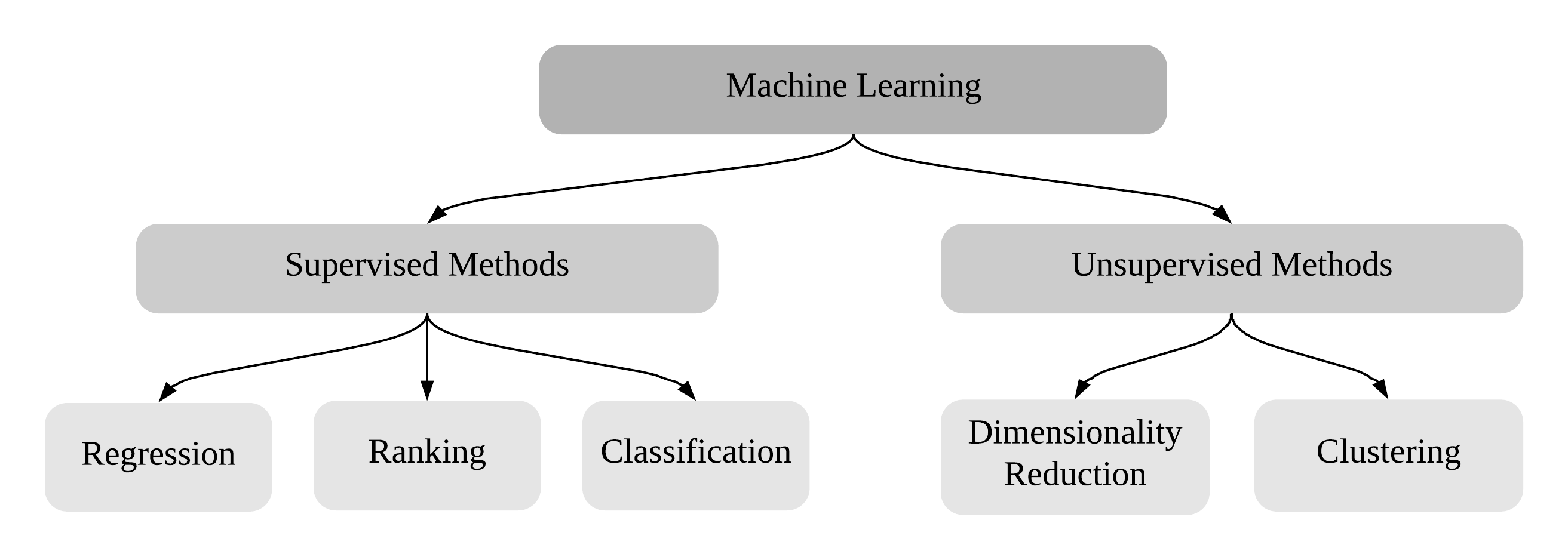
Supervised learning is called so because algorithms using this approach are trained on the data consisting of pairs of the "expected input" - "expected output" type. In other words, being under supervision, an algorithm is explicitly learned to do something specific, hence the name. As an example, handwritten digits classification: for each image of a digit in such a data set, there is a label, whether a given image contains 0, 1 ... or 9.
In the case of unsupervised learning, as you have already guessed, there are no labels - only inputs. This means that an algorithm should find some hidden dependencies in the data and, for example, clusterize it. We can discuss unsupervised algorithms in future posts. But today, in this post we will be talking about neural networks, which are trained with supervision.
Secondly, in the previous post we discussed the basic idea of how perceptron operates. An arbitrary perceptron, being a mathematical function, is designed to perform either a regression or classification task. In the case of a regression task, perceptron can be trained to output any possible (theoretically) output signal, processing some input. Similarly, in the case of a classification task, perceptron can be trained to predict the class label of a given input.
As a part of the technical blog, this post has to express thoughts briefly and clearly, trying to avoid vague wording and concepts. So I would like to elaborate on this a little bit more. Nowadays, plenty of popular media resources speak about neural networks like something "animated". For example, you can often find expressions such as "based on previous experience", "self-learning algorithm" and so on. In fact, of course, there is a human behind everything. A human writes and tests the code that implements various stages of the neural network operation. A human is engaged in the preparation of data and its labeling. Moreover, again, a human "presses a button" to run the process of training, and it is essential to understand, that the training itself is actually automated. That is, a neural network processes the training examples one by one and adjusts its weights accordingly. However, it is worth noting that usually the training process has a lot of different parameters (which will be discussed later), and, of course, a human is responsible for setting them up. Therefore, frankly, it is incredibly difficult to call such a thing fully autonomous, let alone artificial intelligence. Summarizing this up, neural networks are just an algorithm. So let's discuss how this algorithm works.
Multilayer Perceptron
So, suppose you have multiple artificial neurons and some labeled data for solving either a regression or classification task1. As it was explained in the previous post, artificial neurons with the same properties (e.g. with the same activation function) are usually combined into the layers.
A set of such layers forms a neural network, which is usually called a perceptron or a feedforward neural network. The feedforward architecture necessarily has at least one input layer and one output layer that receive and output signals respectively. Depending on how many layers of neurons are between the input and output layers (such layers are usually called hidden), the network can be called a multilayer perceptron or MLP. Just in case, I will repeat and say that it is important that the size of a neural network and number of layers in it do not have primary significance: they all work the same way.
Notation
Let's agree on notation. This part is pretty boring, I do admit it. Nevertheless it will definitely simplify the further conversation, allowing not to repeat the same over and over again.
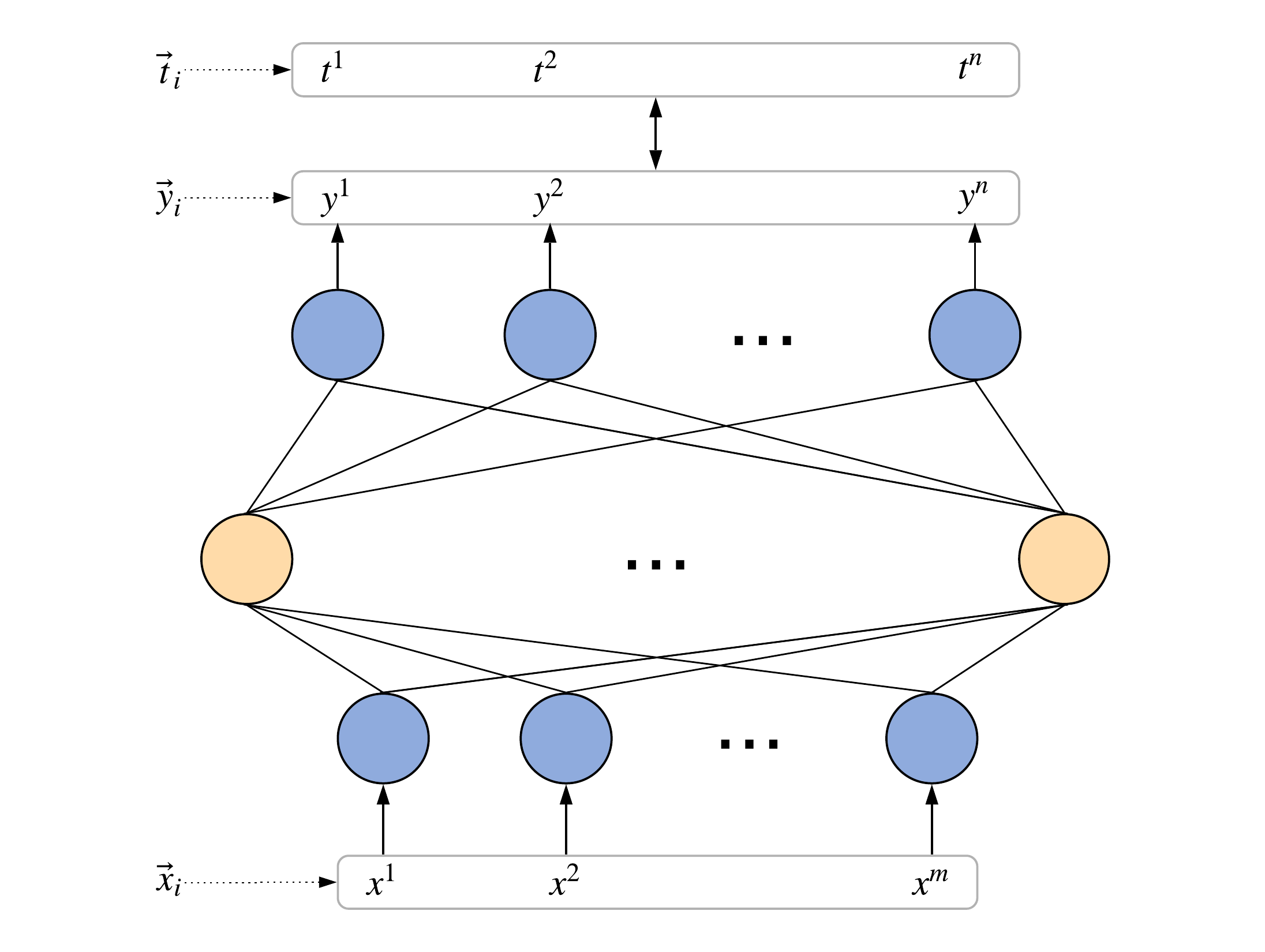
Let pair \((\vec{x}_{i}, \vec{t}_{i})\) stand for \(i\)-th training example, where:
In the case of regression, each expected output signal \(t_{i}^{j}\) could be any real number, whereas for classification it may be either \(0\) (stands for "not \(i\)-th class") or \(1\) (stands for "\(i\)-th class"). Usually, input signals are not limited and can be any real vectors, like pixel brightness values, for example.
As it was already mentioned during our last conversation, a neural network can be viewed as a mathematical function that transforms input signals \(\vec{x}\) into output \(\vec{y}\). And the only thing that this function depends on is the weights of the connections between the neurons (or just weights). A set of all weights and biases of a neural network is conveniently to denote as \(\textbf{w} \). Thus, any neural network is just a function: \(\vec{y} = f_{\textbf{w} }(\vec{x})\).
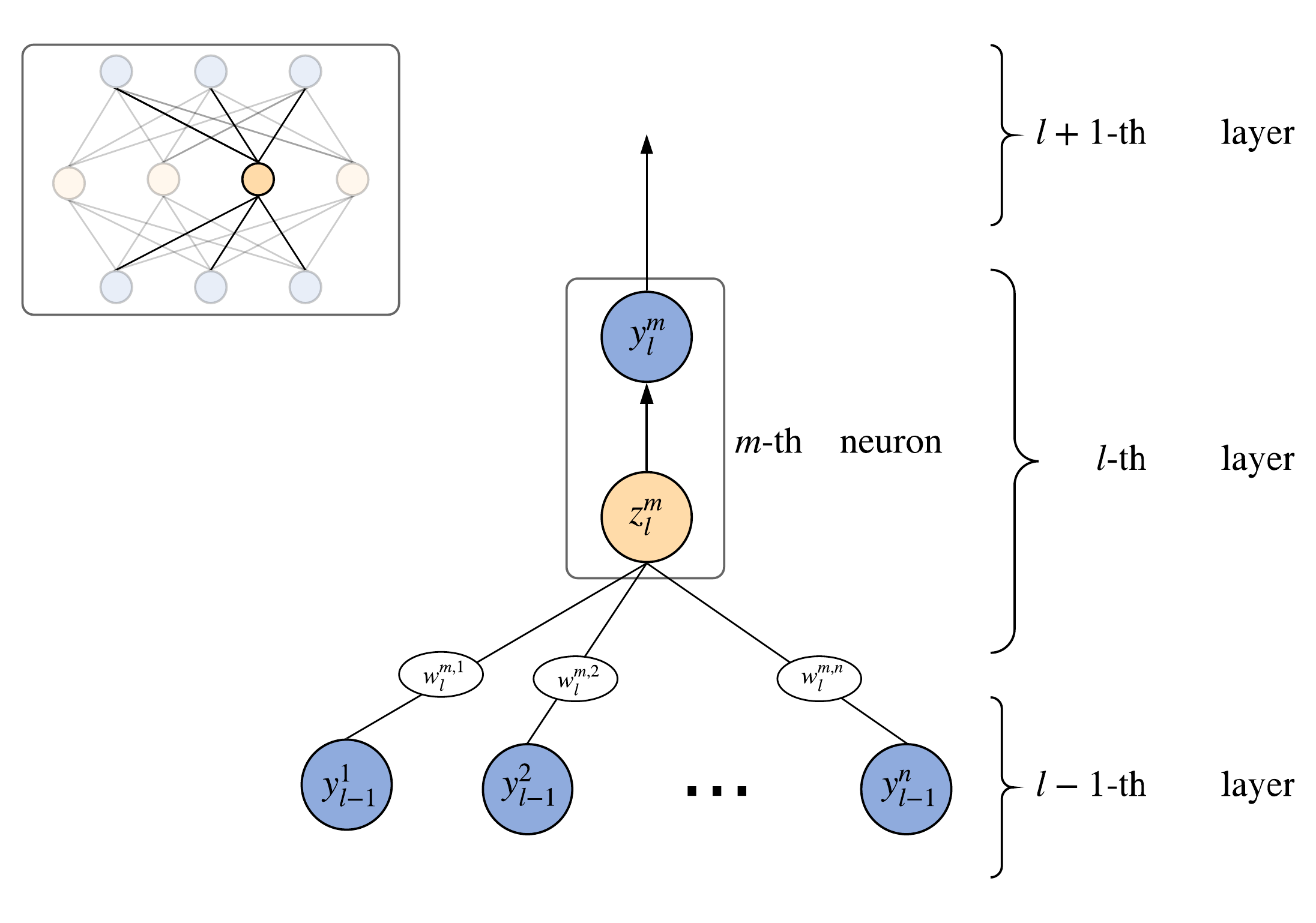
To make a neural network produce desired output, it is necessary to tune its weights. Let's denote them as follows: \(w_{l}^{j,k}\) is the weight of connection between \(j\)-th neuron in \(l\)-th layer with the \(k\)-th neuron of \(l-1\)-th layer. Similarly, if \(\varphi\) is an activation function of the \(m\)-th neuron in \(l\)-th layer, then its output signal \(y_{l}^{m}\) can be computed as a weighted sum (which is called the induced local field \(z_{l}^{m}\)) of all its input signals and a bias \(b_{l}^{m}\): \[ \begin{equation} y_{l}^{m}= \varphi(z_{l}^{m}) = \varphi \left (\sum_{k=1}^{n}(w_{l}^{m,k} \cdot y_{l-1}^{k}) + b_{l}^{m} \right ) \end{equation} \] Here \(n\) is a number of neurons in the previous layer2. As a result, the bottom indices denote the layer number, while the upper indices denote the sequence number of this neuron, starting from the left edge.
Inference
Somebody of you might be interested how exactly output signals are calculated. This process is usually called inference. Actually this process can be implemented in practice in many different ways. Here is one possible way:
In the case of classification, exactly as shown on the illustrations above, if we have \(n\) classes, then we will have \(n\) output neurons. Each neuron outputs a real number from the line segment \([0, 1]\), representing probability that the given input \(\vec{x}_{i}\) belongs to some class \(1\), \(2\), ..., or \(n\). Therefore, NN outputs the probability distribution \(\vec{y}_{i}\) for each \(i\)-th training example:
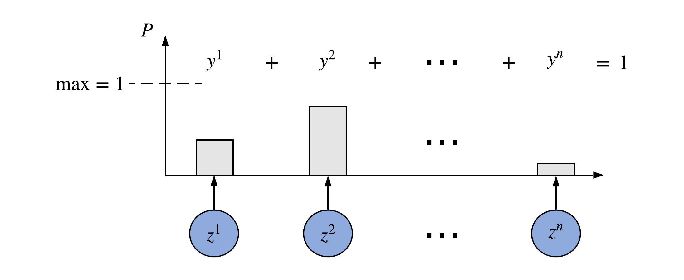
Thus, it is important to ensure, that the output neurons produce signals exactly in the desired range and according to the second probability axiom, the total probability of all outcomes should be equal to \(1\), i.e., \(\sum_{i}^{n} y^{i} = 1\). It is usually achieved by using the softmax function, that basically just normalizes any arbitrary real number vector (raw output neurons' signals in our case) into the vector, whose components will add up to \(1\).
It's also important to note, that in the case of a binary classification problem, it is not needed to have two separate neurons, just because softmax above them will do exactly the same thing as a single neuron would do, using the sigmoid activation function: \(\sigma(x) = (1+e^{-x})^{-1}\). We can easily show this. Since softmax for two classes looks as follows: \[ \lbrace y^{1}; y^{2} \rbrace = \left \lbrace \dfrac{e^{z_{1}}}{e^{z_{1}} + e^{z_{2}}}; \dfrac{e^{z_{2}}}{e^{z_{1}} + e^{z_{2}}} \right \rbrace \] so it can be easily transformed into the following: \[ \lbrace y^{1}; y^{2} \rbrace = \left \lbrace \dfrac{1}{1 + e^{z_{2}-z_{1}}}; \dfrac{1}{1 + e^{z_{1}-z_{2}}} \right \rbrace \stackrel{g=z_{1}-z_{2}}{=} \left \lbrace \dfrac{1}{1 + e^{-g}};\dfrac{1}{1 + e^{g}} \right \rbrace = \lbrace \sigma(g); 1-\sigma(g) \rbrace \] That is it, only single neuron that computes sigmoid is required! If this single neuron outputs 0 (or 1) it can be interpreted that the first (or second) class was predicted.
I especially want to emphasize, that these formulas have concrete rationale. Let's consider two classes \( c_{1},c_{2} \) and some input \(x\) that we want to classify. Then, in accordance with Bayes' theorem, the posterior probability, that \(x\) belongs to \(c_{1}\) can be computed as follows: \[ p(c_{1}|x) = \dfrac{p(x|c_{1})p(c_{1})}{p(x)} = \dfrac{p(x|c_{1})p(c_{1})}{p(x|c_{1})p(c_{1}) + p(x|c_{2})p(c_{2})} \] \[ g = \ln{\left ( \dfrac{p(x|c_{1})p(c_{1})}{p(x|c_{2})p(c_{2})} \right )} \Rightarrow p(c_{1}|x) = \dfrac{1}{1+e^{-g}} \] This is why the sigmoid function looks that way. Similarly, if there are multiple classes, the probability \(p(c_{k}|x)\) is given by: \[ p(c_{k}|x) = \dfrac{p(x|c_{k})p(c_{k})}{\sum_{i} p(x|c_{i})p(c_{i})} = \dfrac{e^{g_{k}}}{\sum_{i} e^{g_{i}}} = \text{softmax}({\vec{g}}); \quad g_{k} = \ln \left (p(x|c_{k})p(c_{k}) \right ) \]
Also, generally speaking, any smooth function can be used for transforming sums of neurons' signals \(\vec{z}\) into the final outputs \(\vec{y}\). We will discuss how this choice affect the training a little later.
In fact, at this stage, this is all we need to know about the inference. Let's continue and go back to how neural networks are trained.
Loss Function
Let's assume that the data set we work with consist of \(N\) training examples: \(\lbrace (\vec{x}_{1}, \vec{t}_{1}), (\vec{x}_{2}, \vec{t}_{2}), \ldots, (\vec{x}_{N}, \vec{t}_{N}) \rbrace\), where each \(c_{i}\) class label corresponds to the respective desired output vector \(\vec{t}_{i}\). If it is a classification problem and there are \(n\) classes, then \(\vec{t}_{i}\in \mathbb{Z}^{n}\) is a probability distribution represented as an one-hot vector: \[ \begin{equation} \vec{t}_{i}=[0,\ldots,\underbrace{1}_{c_{i}:\,i\text{-th example's class label}},\ldots,0] \Leftrightarrow t^{j}_{i} = \begin{cases} 1,&\text{if $j=c_{i}$;}\\ 0,&\text{if $j \ne c_{i}$;} \end{cases} \end{equation} \] If it is a regression problem, then \(\vec{t}_{i}\) is an arbitrary real-valued vector.
As mentioned above, the goal is to somehow teach the neural network to produce the necessary signals \(\vec{t}_{i}\) for a given input \(\vec{x}_{i}\). How to do it? Let's take a closer look at the uppermost layer of an arbitrary perceptron, the so-called output layer. This layer outputs signals \(\vec{y}_{i}\), which ideally should be as close to \(\vec{t}_{i}\) as possible. Ensuring this, the neural network can do what is required of it. Thus, regardless what the task is, it is necessary to somehow adjust NN's weights, that for every \(i\)-th training example the distance, or error, between vectors \(\vec{t}_{i}\) and \(\vec{y}_{i}\) was as small as possible, or more formally3: \[\begin{equation} ||\vec{t} - \vec{y}|| \rightarrow 0,\quad \forall i = \overline{1,N} \end{equation} \]
So, with the given weights \( \textbf{w} \), a neural network produces specific errors for each training example. So it is convenient to combine them all together to estimate how "good or bad" the neural network works on a given data set at the current moment with the given weights. Exactly at this point the definition of the loss function arises: \[\begin{equation} L = \dfrac{1}{N} \sum_{i}^{N} ||\vec{t}_{i} - \vec{y}_{i}|| \end{equation} \] This is the average sum of all errors produced by the neural network for each training example. The sum is averaged because we don't want the loss function value to depend on the number of examples used. Using definition of the loss function \((3)\), expression \((2)\), which stands for the goal of a neural network training, can be generalized as follows: \[ \begin{equation} \textbf{w}^{*} \equiv \text{optimal}\,\, \textbf{w} = \operatorname*{argmin}_{\textbf{w} } \left ( L \right) \end{equation} \] In fact, this is the answer to the question that we asked earlier:
In order to train a neural network, it is necessary to find a global minimum of an appropriate loss function. A point \( \textbf{w}^{*} \), where the loss function reaches its global minimum, gives a set of optimal weights4.
Theoretically, these optimal weights will allow the neural network to produce desired signals for the given training data set. However, as you know, the reality is ugly and therefore, the above case is not always working in practice. Sometimes it is too hard (and/or computationally expensive) to find the global minimum. Sometimes a neural network that was trained very well on some data, doesn't give a good performance on the previously unseen examples. There are many different restrictions and rules, applicable for the training process, and without following them it's easy to get an absolutely useless neural network for practical purposes. But let's talk about these nuances a bit later, now - we need to come back to the loss function.
By its definition, any loss function depends only on the weights of the network and training data. Therefore, in terms of the output layer neurons, minimization of a loss function "penalizes" each output neuron, if they don't produce exactly expected signals. And because these output neurons depend on all underlying neurons' signals, this penalization applies to every neural network's weight.
For example, in the case of a quadratic loss function, it can be computed as follows (why? we will talk about it a bit later): \[ L = \dfrac{1}{2N} \cdot \left ( \underbrace{\overbrace{(t_{1}^{1}-y_{1}^{1})^{2}}^{\textit{first neuron}} + \ldots + (t_{1}^{n}-y_{1}^{n})^{2}}_{\textit{first example}} + \cdots + \underbrace{||\vec{t}_{N}-\vec{y}_{N}||^{2}}_{N\textit{-th example}} \right ) \]
Theoretical Justification
Before turning to the question of how to find the global minimum of the loss function, I would like to emphasize that in addition to the purely geometric considerations, there are other approaches to derive the loss function. Probability theory and mathematical statistics can be used to theoretically prove that all we've gotten so far is correct and it actually works.
Let's denote input examples data set as \(\mathcal{X}\) and class labels set as \(\mathcal{C}\). Let's also consider an arbitrary neural network with weights \(\textbf{w} \) that is used for a classification task \(\mathcal{X} \rightarrow \mathcal{C}\) to be trained on the data set \((\mathcal{X}, \mathcal{C}) = \lbrace (\vec{x}_{1},c_{1}), \ldots, (\vec{x}_{N},c_{N}) \rbrace \). For brevity, we will denote the data set as \(\mathcal{D}\).
We can assume, that all input examples \(\vec{x}\) and output class labels \(c\), which make the training set, are actually samples obtained using two random distributions, i.e., we can consider that \(\chi \, : \Omega \rightarrow \vec{x} \in \mathcal{X}\) and \(\tau \, : \Omega \rightarrow c \in \mathcal{C}\) are two random variables, which represent random samples from \(\mathcal{X}\) and \(\mathcal{C}\) sets correspondingly. Let's also assume, that the joint random variable \((\chi, \tau) \, : \Omega \rightarrow (\mathcal{X}, \mathcal{C})\) has joint probability distribution, with the density that we will denote as \(p_{d}(\vec{x}, c)\). This distribution is often called the empirical distribution.
Having clarified the notation, it is time to move to the tastiest! The goal of any supervised machine learning algorithm (more precisely - any discriminative model), including the neural network we are considering, is to build a model that can estimate empirical distribution \(p_{d}(\vec{x}, c)\). How to express this idea in the language of probability theory and mathematical statistics?
First, let's define what a neural network does from a probabilistic point of view. As we've already discussed above, the output layer of the neural network predicts probability distribution over the class labels. In probability theory terms, this distribution can be interpreted as the multidimensional conditional probability that given example \(\vec{x}\) belongs to some class \(c\). This conditional probability is usually denoted as \(p_{\textbf{w}}(c|\vec{x})\) or \(p(c|\vec{x}, \textbf{w})\), because the neural network's output \(\vec{y} = f_{\textbf{w} }(\vec{x})\), used to predict this class label \(c\), also depends on the weights \( \textbf{w} \).
Secondly, we need to imagine that the classification of each individual example is an experiment, which is carried out using our NN model (this is similar to the classical example of coin flipping). Thus, having conducted \(N\) independent experiments, we are able to compute the probability \(p_{\textbf{w}}(\mathcal{D})\) of observing the data set \(\mathcal{D}\). For a fixed set of weights, this probability is equal to the so-called likelihood function \(\mathcal{L}\, : \Omega \rightarrow \mathbb{R}\), or simply the likelihood. The likelihood shows how plausible the selected NN's weights \(\textbf{w}\) are, given the observed data \(\mathcal{D}\): \[ \begin{equation} \mathcal{L} \equiv \mathcal{L}_{\textbf{w}}(\mathcal{D}) = p_{\textbf{w}}(c_{1},\ldots,c_{N}|\vec{x}_{1},\ldots,\vec{x}_{N}) = p_{\textbf{w}}(\mathcal{D}) \end{equation} \]
Let's additionally assume that all training examples are independent and drawn uniformly from the empirical distribution \(p_{d}(\vec{x}, c)\), so they are i.i.d.. This will allow us to compute the aforementioned likelihood as for independent events5, using our model: \[ \begin{equation} \mathcal{L} = \prod_{i=1}^{N}p_{\textbf{w}}(c_{i}|\vec{x}_{i}) \end{equation} \]
So we are given a fixed data set \(\mathcal{D}\), a model that can estimate individual conditional probabilities \(p_{\textbf{w}}(c|\vec{x})\), and the likelihood function \(\mathcal{L}\) to be computed by this model for this data set. How to combine this all together? According to the definition, the higher the likelihood is, the higher the probability \(p_{\textbf{w}}(\mathcal{D})\) is. Thus, similarly to \((5)\), weights \( \textbf{w}^{*} \) which will give the highest likelihood are the optimal weights: \[ \begin{equation} \textbf{w}^{*}= \operatorname*{argmax}_{\textbf{w}} \mathcal{L} \end{equation} \] Such an approach is called maximum likelihood estimation (or MLE) and it is proved that the estimate it provides for \(N \rightarrow \infty \) is consistent and unbiased. That is why MLE results are reliable enough to be used in practice.
As shown above, we don't actually need to worry about the actual likelihood value. The only thing that matters is where this likelihood has a maximum. It simplifies everything significantly. Watch the hands carefully!
Let's take advantage of the fact that the extrema of a function \(f(x)\) and its composition with an arbitrary monotonic function \(g(f(x))\) are the same, so let's use the logarithm (which is monotonic, of course) to simplify \((7)\) and \((8)\): \[ \textbf{w}^{*}= \operatorname*{argmax}_{\textbf{w}} \hat{\mathcal{L}}; \qquad \hat{\mathcal{L}} = \log{\mathcal{L}} = \sum_{i=1}^{N} \log{p_{\textbf{w}}(c_{i}|\vec{x}_{i})} \] Due to the same reason, optimal weights point won't be changed even if we will multiply the likelihood by some constant value, therefore we can average \(\hat{\mathcal{L}}\): \[ \hat{l} = \dfrac{\mathcal{L}}{N} = \dfrac{1}{N} \sum_{i=1}^{N} \log{p_{\textbf{w}}(c_{i}|\vec{x}_{i})} \] Does this expression ring a bell?! Taking into account the law of large numbers (i.e., in the case when \(N \rightarrow \infty \)), \(\hat{l}\) defined above becomes nothing else than the expected value of \(p_{\textbf{w}}(c|\vec{x})\) with respect to \(p_{d}(c|\vec{x})\). This fact is usually denoted by: \[ \hat{l} \approx \mathbb{E}_{\vec{x} \sim p_{d}(c|\vec{x})} [ \log{p_{\textbf{w}}(c|\vec{x})}] \] Thus, we finally have: \[ \begin{equation} \textbf{w}^{*} = \operatorname*{argmax}_{\textbf{w}} \hat{l} = - \operatorname*{argmin}_{\textbf{w}} \mathbb{E}_{\vec{x} \sim p_{d}(c|\vec{x})} [ \log{p_{\textbf{w}}(c|\vec{x})}] = \operatorname*{argmin}_{\textbf{w}} H(p_{d}, p_{\textbf{w}}) \quad \blacksquare \end{equation} \] , where \(H(p_{d}, p_{\textbf{w}})\) is called the cross-entropy between the empirical distribution \(p_{d}\) and the model-estimated one, \(p_{\textbf{w}}\). \(H(p_{d}, p_{\textbf{w}})\) is basically a measure of how close these two distributions are. Consequently, maximization of \(\hat{l}\) given by \((9)\) makes the conditional probability distributions \(p_{\textbf{w}}(c|\vec{x})\), produced by the neural network, maximally close to the desired ones \(p_{d}(c|\vec{x})\). This confirms our intuitive hypothesis put forward a little earlier - see \((3,4,5)\). Furthermore, since we need to minimize the cross-entropy, it can be considered as the loss function: \(L = -\hat{l} = H(p_{d}, p_{\textbf{w}})\). By the way, we can prove this hypothesis and achieve the same results considering the Kullback–Leibler divergence between \(p_{d}\) and \(p_{\textbf{w}}\).
It is important to take into account that all formulas above are given considering that distribution \(p_{d}(\vec{x}, c)\) is actually an empirical approximation of the real data-generating distribution \(\hat{p}_{d}(\vec{x}, c)\). Therefore, the process which is expressed through \((9)\) is also called the empirical risk minimization. What we ideally want is to compute MLE using the real distribution \(\hat{p}_{d}(\vec{x}, c)\) (i.e., representing all possible inputs and outputs) rather than the finite \(p_{d}(\vec{x}, c)\), which is limited by a given data set. Unfortunately, in most of the cases, the true distribution is unknown, so the approximation is needed. Otherwise, instead of machine learning, methods for computing integrals \(\mathbb{E}_{\vec{x} \sim \hat{p}_{d}(c|\vec{x})} [ \log{p_{\textbf{w}}(c|\vec{x})}] \) would have been actively developed. This nuance is one more assumption in addition to those, which we have already mentioned earlier. We will further discuss it in the next post.
Key Findings
Let's summarize the above:
Any supervised-model training is the process of maximizing the data-set likelihood, given by the model-estimated probability distribution, that is equivalent to minimizing the respective cross-entropy.
How is it used in practice? Formulas above are utilized to build the loss-functions needed to train neural networks for a variety of tasks. Here are some most popular examples.
...
Now we have the thing that we need to be aware of while studying neural networks: understanding of how and where to get the loss function and why it is needed. I would even say that everything else, such as finding the optimal weights, knowing the loss function, is just a matter of applying mathematical methods in practice. We will talk about them in the next post. Thanks for reading this!
Notes
- In practice, classification task is more common, so to simplify the reasoning we will consider only it. In the case of regression, almost all considerations remain the same, and we will separately specify exceptions.↩
- For the output signals, indices denoting training example number are omitted for brevity.↩
- \(||\cdot||\) usually denotes any metric on a vector space, but in this post we assume that it is a regular Euclidean distance, i.e., \(||\vec{x}|| \equiv ||\vec{x}||_{2} = \sqrt{\sum_{i}^{n} x_{i}^{2}} \). ↩
- Take a look at these notes if you want to refresh your knowledge about extrema.↩
- So far we have already assumed two different things: data-generating distribution is made of two independent probability distributions and the training examples are i.i.d., and we have many training examples to consider \(N \rightarrow \infty \) to be true. ↩
- This assumption is quite true in accordance with CLT. ↩
- This forumaltion can be thought as a Bernoulli trial, where \(j\)-th neuron predicts that the input belongs or doesn't belong to \(j\)-th class with some probability \(y^{j}\) or \(1-y^{j}\) respectively. ↩