Multilayer Perceptron.

Part III: Regularization.

Although we have already touched upon this topic in the previous post, I would still like to give more details on how various factors, like the training data size, for instance, may affect the real trained ML model quality and in addition discuss some important nuances associated with the training of neural networks.

Trained Model Quality

Last time, we found out that while estimating model parameters and constructing the approach to compute them, the following two important assumptions were used:

Training examples are independent and identically distributed,

The number of training examples \(N\) is large.

While the first assumption is surmountable in practice, because it is relatively easy to make a data set with different and diverse examples, the second one always requires a lot of effort. Of course, the fulfillment of these requirements does not guarantee that the trained model will ideally cope with the task of processing previously unseen examples. However, on the other hand, ignoring these requirements can adversely affect the model used in practice. Let's consider the following example of how this can manifest itself.

It is often the case that a trained model performs very well on the training data, but it works poorly¹ (or doesn't work at all) on the so-called validation data, that is, those examples that the model has never seen before. This validation data set is used as an indicator of the model's generalization ability.

Broadly speaking, assuming the the model has enough capacity (i.e. it is large and complex enough), then the most probable cause of the poor generalization quality is because the empirical joint probability distribution of the data \(p_{d}(\mathcal{D})\) represents the real data distribution \(\hat{p}_{d}(\mathcal{D})\) too roughly (see this post where this notation was introduced). This usually happens due to the lack of training examples or if they are not diverse enough. Well ...

What Do We Do?

Using the additional knowledge about parameters of a model that we train can significantly help the cause. In the case of a neural network, these parameters are all neurons' weights and biases \(\textbf{w} \). Such additional knowledge is usually called "a priori information", hence the name prior probability distribution \(p(\textbf{w})\). This distribution is used to refine the approximation of model parameters. How to use that? Let's try to look at this problem from a probabilistic point of view. To do so, it would be great to consider the full posterior distribution \(p(\textbf{w}|\mathcal{D})\) of weights \(\textbf{w}\) for a given data set \(\mathcal{D}\). We can write an expression for \(p(\textbf{w}|\mathcal{D})\) using the Bayes' theorem: \[ \underbrace{p(\textbf{w}|\mathcal{D})}_{\text{posterior}} = \dfrac{\overbrace{p_{\textbf{w}}(\mathcal{D})}^{\text{likelihood}} \, \cdot \, \overbrace{p(\textbf{w})}^{\text{prior}}}{\underbrace{p(\mathcal{D})}_{\text{marginal likelihood}}} \] Here \(p(\mathcal{D})\) is the total probability of having a data set \(\mathcal{D}\) considering all possible weights values - the so-called marginal likelihood or the evidence. It is difficult to calculate \(p(\mathcal{D})\) as the calculation would involve a large sum, but on the other hand \(p(\mathcal{D})\) doesn't depend on the weights \(\textbf{w}\) being an integral variable. Therefore, as in the case of the maximum likelihood estimation, we are not concerned with a specific value of \(p(\textbf{w}|\mathcal{D})\). We only care about the point \(\textbf{w}^{*}\) where this posterior probability has a maximum value, therefore, we have: \[ \begin{equation} \textbf{w}^{*} = \operatorname*{argmax}_{\textbf{w}} p(\textbf{w}|\mathcal{D}) = \operatorname*{argmax}_{\textbf{w}} \left[p_{\textbf{w}}(\mathcal{D})p(\textbf{w})\right] \end{equation} \]

This principle is called maximum a posteriori estimation or MAP. If we had not had information on how weights should look like, then we should have considered \(p(\textbf{w})\) as a constant. Consequently, the estimate \((1)\) would have been equal to the maximum likelihood estimate value, because in this case \(p(\textbf{w})\) has no affect on the \(p(\textbf{w}|\mathcal{D})\) maximum.

Based on the first post results, we may assume that \(p_{\textbf{w}}(\mathcal{D}) \approx \prod_{i=1}^{N}p_{\textbf{w}}(c_{i}|\vec{x}_{i})\), thus using this approximation and applying the logarithm, equation \((1)\) can be rewritten as follows: \[ \begin{equation} \textbf{w}^{*} = \operatorname*{argmax}_{\textbf{w}} \left[p_{\textbf{w}}(\mathcal{D})p(\textbf{w})\right] = \operatorname*{argmax}_{\textbf{w}} \left[\dfrac{1}{N} \sum_{i=1}^{N} \log{p_{\textbf{w}}(c_{i}|\vec{x}_{i})} + \log{p(\textbf{w})}\right] \end{equation} \] The first term is the well known negative cross-entropy \(-H(p_{d}, p_{\textbf{w}})\) between the model and data probability distributions, whereas the second term, usually denoted as \(-R(\textbf{w})\) (minus is important) is the so-called regularization term, and that is why the process \((2)\) of finding optimal weights \(\textbf{w}^{*}\) is referred to as the training with regularization. Combining everything together, similarly to \((9)\), we obtain the following general expression for the loss function: \[ \begin{equation} L_{\text{reg}} = \underbrace{H(p_{d}, p_{\textbf{w}})}_{L} + R(\textbf{w}) \end{equation} \quad \blacksquare \]

This is how the knowledge of weights distribution affects the training of neural networks — it results in the addition of the extra term to the loss function. Let's look at some examples below and discuss why this term is important and how it works.

\(L_{2}\)-regularization

For example, if during the training procedure we want to "encourage" small weights (this technique is called weight decay), then we can assume that the prior \(p(\textbf{w})\) is given by the normal distribution \(\mathcal{N}(\textbf{w}; 0, \textbf{I}^{2}/\lambda)\), where \(\textbf{I}\) is the identity matrix with corresponding dimensions and \(\lambda \in [0,+\infty)\) is a manually chosen hyper-parameter. In this case: \[ R(\textbf{w}) = -\log{p(\textbf{w})} \propto -\log{e^{-\lambda \cdot \textbf{w}^{\top} \textbf{I} \cdot \textbf{w}}} = \lambda ||\textbf{w}||_{2}^{2} = \lambda \cdot (w_{1}^{2} + w_{2}^{2} + \ldots) \] This is why such type of regularization is often called \(L_{2}\)-regularization. The term \(||\textbf{w}||_{2}^{2}\) facilitates only small weights, thereby making the final value of \(||\textbf{w}^{*}||\) less. Below there is an example for the loss function that depends only on two variables: \(L=L(w^{1},w^{2})\). The surface \(L_{\text{reg}}\) of the loss function with \(L_{2}\)-regularization is shown in green color:

Such a simple idea has proven to be very efficient in practice. Moreover, various neural network's layers weights can be regularized differently, i.e., if multiple sub-distributions form the overall prior. This can also help to improve the NN's performance.

In the conclusion of this section, it is necessary to understand how the addition of regularization affects the technical side of the optimization. To do this we just need to choose the regularization term, for example, the aforementioned \(R(\textbf{w}) = \lambda ||\textbf{w}||_{2}^{2}\), and compute the derivative of \((3)\) with respect to the weights, so: \[ \nabla L_{\text{reg}} = \nabla L + 2 \lambda \textbf{w} \Rightarrow \Delta \textbf{w}_{\text{reg}} = - \eta \cdot \nabla L_{reg} = \Delta \textbf{w} - 2 \lambda \eta \textbf{w} \] This means that every weight's update \(\Delta w_{ij}^{t+1}\) decreases by a certain regularization value \(- 2 \lambda \eta w_{ij}^{t}\). This results in pushing the values of the optimal weights towards the origin.

\(L_{1}\)-regularization

In the vast majority of cases, dealing with optimization problems, one has to deal with multivariable functions - the concept of vector spaces appears. Also, it happens often that loss functions in machine learning are measurable in \(L_{p}\) spaces. This is why the following two popular types of norms are used for regularization: \(L_{1}\) and \(L_{2}\). All right, let me stop speaking formally... The second regularization term type has just been considered as an example above, so let's talk a bit about the first one.

In fact, the difference is not fundamental in the approach but is quite noticeable in the results obtained. First, let's take a look at the corresponding regularization term: \[ R(\textbf{w}) = \lambda \cdot ||\textbf{w}||_{1} = \lambda \cdot (|w_{1}| + |w_{2}| + \ldots) \] This expression could be also obtained using the Laplace distribution \(p(\textbf{w}) \propto e^{-\lambda |\textbf{w}|}\) in the way as we just did before for \(L_{2}\)-regularization and the normal distribution. Well, now we can compute the update for some arbitrary weight \(w\) as follows²: \[ \Delta w_{\text{reg}} = \Delta w - \lambda \eta \cdot \text{sgn}(w) \] Thus, regardless of the weight absolute value \(|w|\), its update \(\Delta w_{\text{reg}}\) is always non-negative (even if \(\Delta w = 0\)) both for any positive or negative value. Therefore \(L_{1}\)-regularization results in facilitation of zero weights, because in this case \(L_{\text{reg}}\) would be closer to its minimum³. Ultimately, this regularization leads to a higher sparsity of the weights obtained at the end of the training. Such a consequence can be interpreted as the feature filtering, i.e., the model essentially learns to ignore most of the useless features. This is how \(L_{1}\)-regularization can help neural networks to understand the features of the data better.

Other Techniques

Nowadays, the concept of regularization is more general than a simple tweaking out of the loss function. In a broader sense, regularization refers to any method aimed at overcoming the effect of overfitting mentioned above. There are a couple of examples:

Weights Initialization

As was discussed in previous posts, the weights of a neural network can be initialized randomly. Of course, even being simple and intuitive, this method does not always work well. Although this is an incredibly interesting topic, here I would like to mention only the main idea of how the proper weights initialization can help. Generally speaking, it may help to accelerate the passage of signals through the neural network in both directions, that is, when calculating the output signals and updating the weights using the back-propagation algorithm.

Here is an example. One common approach, called Xavier initialization, suggests to initialize all \(l\)-th layer's weights \(w_{l}\) using the uniform distribution with coefficients proportional to the inverse square root of the number \(n\) of neurons in \(l\)-th and \(l+1\)-th layers together:

\[ w_{l} \sim U \left [ -\sqrt{\dfrac{6}{n_{l}+n_{l+1}}}; \sqrt{\dfrac{6}{n_{l}+n_{l+1}}} \right ] \]

As it turned out, this heuristic does help to accelerate the training and improves the generalizing ability. To know why this works, I'd recommend taking a look at the primary source.

Batch-normalization

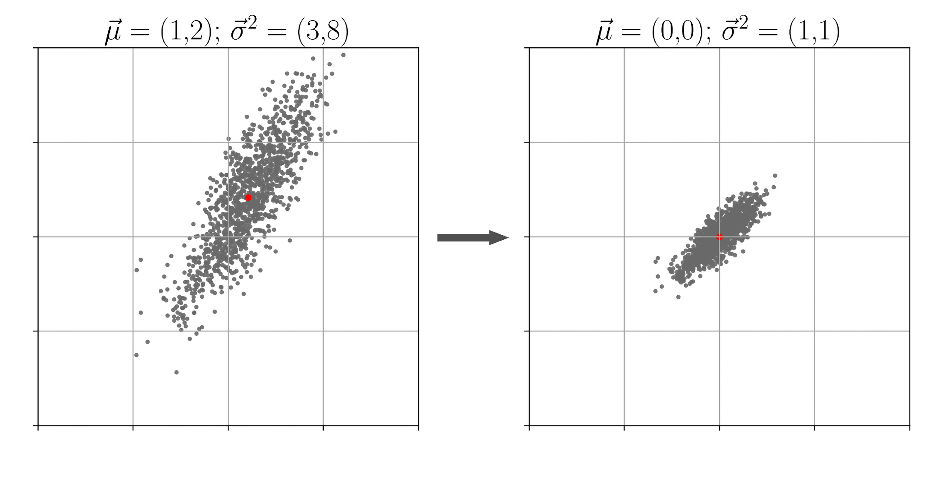
The authors of this research found a way to speed up the training and help the loss to converge to even a lower point, while using a mini-batch gradient-based backpropagation algorithm. The idea is to apply linear data transformation to every neuron of a neural network. Let's consider a neuron's induced local fields \(z_{1},\ldots,z_{i},\ldots,z_{|\pi|}\) collected over a batch \(\pi\). One can normalize these signals based on the statistical properties of the batch:

\[ z_{i} := \gamma \cdot \left ( \dfrac{z_{i} - \mu}{\sqrt{\sigma^{2} + \varepsilon}} \right ) + \beta, \quad \forall i \in \pi \] \[ \varepsilon, \gamma, \beta \in \mathbb{R}; \, \mu = \dfrac{1}{m}\sum_{i=1}^{|\pi|}z_{i}; \sigma^2 = \dfrac{1}{m}\sum_{i=1}^{|\pi|}(z_{i}-\mu)^{2}; \]

\(\gamma\) and \(\beta\) are two hyperparameters which are optimized during the training, whereas \(\varepsilon > 0\) is a fixed parameter that prevents the division by zero. This technique is called batch normalization⁴. During the classification time, the neural network uses values of \(\mu\) and \(\sigma\), which were averaged among all training batches.

Utilizing batch normalization, you should keep in mind that it requires additional overhead costs both in time and in memory. For example, each neuron to which this procedure applies must store four additional variables: \(\gamma, \beta, \mu, \sigma\). And this is at least 16 bytes on modern computers.

All these statistical manipulations normalize the expectation and variance of the gradients. Thus higher learning rates are becoming stable enough. This, in turn, has a positive effect on the characteristics of the trained model and the time required to train it.

Data Augmentation

Here everything is pretty much straightforward, at least from the practical point of view. The idea is to have more data for the training. By "more" in this context, additional data generated from already existing examples is meant. Yep. That simple. "Why?" you may ask. This question has been already answered above: the more data you have and the more diverse it is, the better the real-world data distribution a neural network will learn.

For example, in speech recognition tasks, the addition of various noises is often used as the augmentation, such as applause, distant voices, or street sounds in the background. For the graphical problems, distortion, warping, rotation, and scaling of images are commonly used to augment the training data set. Thus, the neural network will be able to generalize its knowledge to a broader range of previously unseen examples. So yet another passenger's face will be registered at the airport, and a camera will recognize one more dirty license plate at the entrance to the toll bridge.

Early Stopping

Suppose you have enough data, then you most likely have the opportunity to divide all the available data into two representative parts, for example, with the ratio of 7:3 or 4:1. A large part, called the training set, is (please make a guess...) used for training. At the end of each epoch, while a neural network is trained, the loss function value is calculated on the second, the remaining part of the data, called the validation set. If you plot the dependency of the training and validation losses on the number of epochs passed, the typical (smoothed) behavior of these two curves will look as follows:

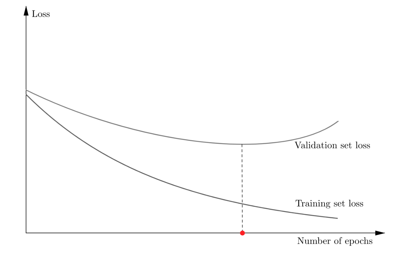
The neural network performance on the validation set is becoming worse and worse after some specific number of epochs. Therefore, one should keep an eye on these two curves throughout the entire training process in order to choose the proper point in time when to stop the training. This procedure is called the early stopping, and even being a common-sense demonstration, it is usually considered as a regularization technique⁵.

Ensemble of Models

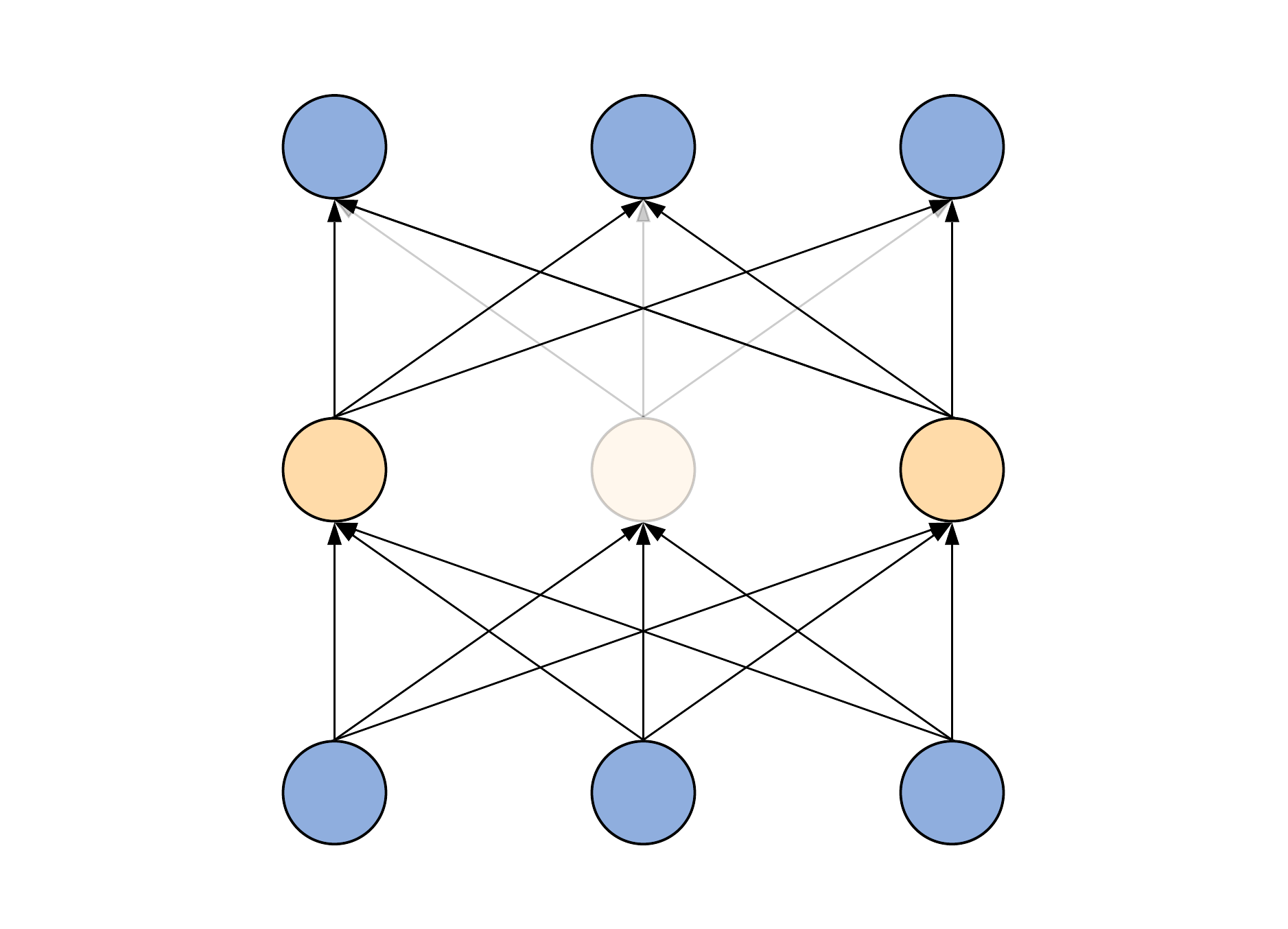
Let's consider an arbitrary neural network. Also, let's consider, two more copies of the same architecture and change something a little bit in each of them — for instance, the number of neurons in layers:

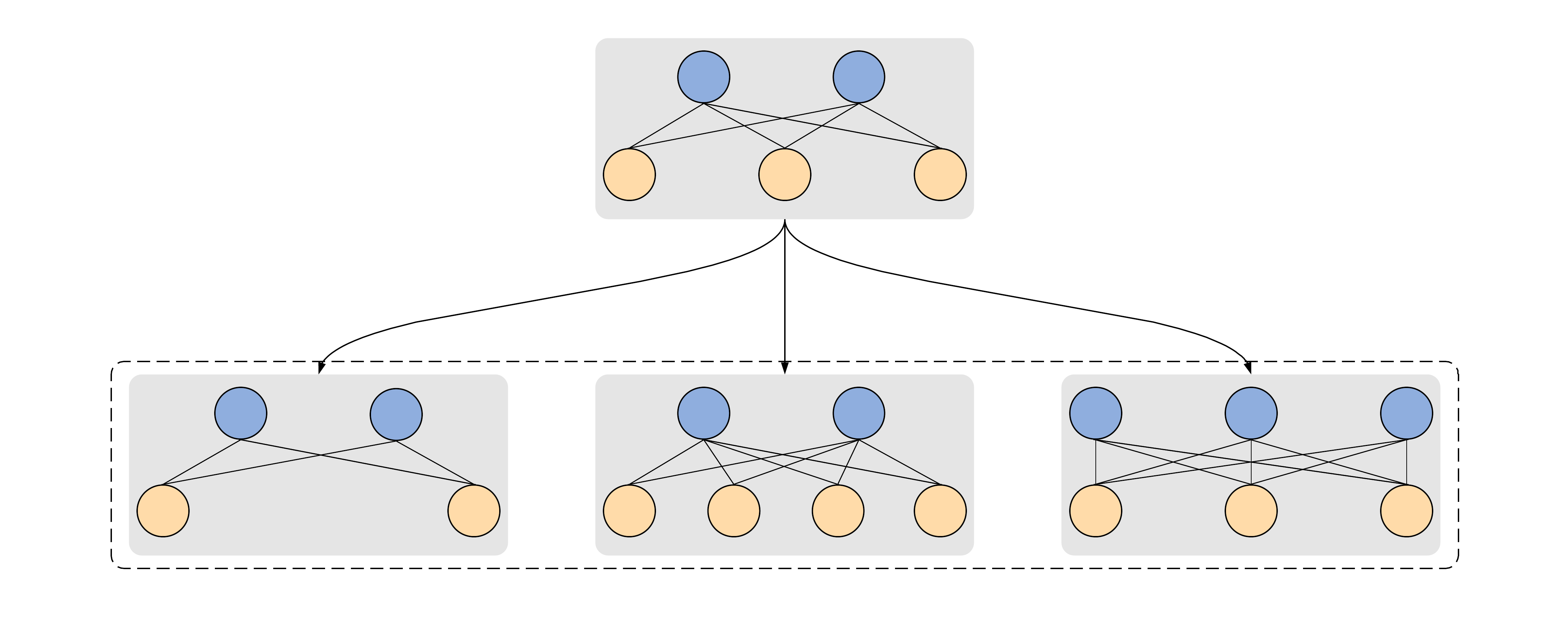
Now let's train all these three neural networks to perform the same task, say, recognize cats on pictures, namely, say yes or no depending on the presence of a cat in the image. Then we can take all three trained copies and utilize them to classify some arbitrary pictures. To do so, we assume that there is a cat if and only if all three networks agree with this, and there is no cat if at least one network disagrees with that. This kind of unification is called an ensemble. This approach is pretty much expensive, but it often helps to achieve higher accuracy and lower false positive rate for various classification problems.

The existence of multiple copies of the same neural network which are trained and used for classification together works as a regularization. The randomness of the initial weights initialization and slightly different architecture characteristics lead to more accurate learning of the different data features. For example, the first model has learned to predict only one part of the classes well, while the second one has learned only the remaining classes quite well. Almost like in everything, teamwork is better and more effective than the work of one.

Dropout

How can one make an ensemble of models to be more efficient in practice? The first thing that comes to mind is to try to train many models at the same time. Here comes the dropout approach! The idea is in switching off a certain number of neurons randomly during every forward-backward pass, that is, with every new batch, thereby simply excluding these neurons both from the output signal calculation and weights update.

The only thing that the user should regulate is the so-called dropout rate \(p\) that states for the percentage of neurons, which will be randomly turned off in every network's hidden layer. Consequently, the probability that a given hidden neuron will be turned on during an arbitrary training step is given by \(q = 1-p\). Therefore, during the classification, in order to emulate that the neural network actually was trained as an ensemble of multiple models, one need to multiply every hidden layer neuron's output signal by \(q\). This is equivalent⁶ to the division of all output signals by the same value \(q\) during the training time. In practice, this approach is actually more preferable since it doesn't require any additional actions during the classification time.

Of particular note is the efficiency of dropout in reducing the overfitting. Various researches have proved that dropout remarkably increases the generalization ability of almost any arbitrary neural network architecture used almost for any task.

...

Obviously, regularization is not given for free. The price of the model's generalization ability improvement is increased computational complexity and additional memory consumption. Nevertheless, for large production ML-powered systems, the generalization ability of a model has a higher priority over the training time reduction. Therefore, the use of various regularization methods is highly recommended.

Notes

---

1. Manifestations of such behavior is combined under a general term overfitting.↩
2. \(\text{sgn}(x)\) is the so-called sign function.↩
3. See this nicely written "Deep Learning Book"'s chapter in order to find the strict mathematical proof of such conclusion.↩
4. One important note. Sometimes, it's more efficient to apply batch normalization after the activation function, i.e., to the neuron's output signal \(y_{i}\), and not to the induced local field \(z_{i}\). In most cases, a specific configuration is selected experimentally.↩
5. I recommend referring to this comprehensive article for other effective ways of model selection.↩
6. Assuming that \(P\) is a function that randomly switches off a given neuron with probability \(p\), the regular dropout will work as follows: \(\tilde{y}_{\text{train}}=P \cdot y_{i}\) and \(\tilde{y}_{\text{test}} = q \cdot y_{i}\), whereas inverted dropout works slightly differently: \(\tilde{y}_{\text{train}}= (1/q) \cdot P \cdot y_{i}\) and \(\tilde{y}_{\text{test}} = y_{i}\).↩

---